Building a simple deterministic model
Last updated on 2025-11-11 | Edit this page
Overview
Questions
- How to build a simplified model of Zika?
Objectives
At the end of this workshop you will be able to:
Recognize how a simple deterministic model is built using ordinary differential equations.
Identify relevant parameters for modeling vector-borne disease (VBD) epidemics.
Learn how to create a diagram for a compartmental model
Translate mathematical equations for a deterministic model into R code.
Use model simulations to explore transmission scenarios and the potential impact of interventions.
Prerequisite
This unit has the following prerequisites:
- Introduction to epidemic theory
Table of Contents
|
Topic 1: Vector-borne diseases - Biology of the vector-borne disease - Vector biology, Zika virus, diagnostics, and intervention Topic 2: Review - What is a simple deterministic model? Topic 3: Simple SIR Model for Zika Topic 4: Developing diagrams and equations of the Zika model Topic 5: Elaborating the parameter table of the simple Zika model Topic 6: The Zika model in R Topic 7: Parameterization of control interventions for Zika |
Introduction
In this unit we will address the construction of a simple deterministic model, specifically for the Zika virus, a disease that triggered a major epidemic in Latin America and the Caribbean, and which was declared a public health emergency of international concern. Using previous knowledge of epidemic theory, we will build a deterministic SIR-type model that incorporates demographic aspects.
To build this model, we will learn about the dynamics of interaction between humans and vectors, as well as the fundamental parameters that govern these biological processes. By constructing a diagram, we will examine these relationships and formulate equations that describe the behaviour of the system. These equations will be the basis for simulating the model in the R programming language. In turn, we will propose and model intervention strategies.
Through the analysis of the model, we will evaluate the potential impact of this epidemic on society, contextualising some of these interventions in Latin America. In addition, we will reinforce and apply key themes such as: SIR model, Herd immunity, Parameters and control interventions (spraying, bed nets and vaccination) for a Vector Borne Disease (VBD).
Topic 6: Zika model in R
In this section we will put to use the knowledge acquired about Zika, the mechanisms involved in transmission and the model equations. The aim is to build it in R.
The only package required for the modelling is deSolve, which allows us to solve the differential equations. Additionally for data handling and plotting the results we recommend using tidyverse and cowplot.
6.1 Practical start in R
To start our practice in R please open a project of Rproject and create a new document. In this document we must load the functions we have just explained. If you have difficulties with this process, please review the unit Introduction to R.
install.packages(deSolve) # deSolve package for solving differential equations
Once you have installed the deSolve package please load the packages with the following lines of code, copy them into your R script and run them.
R
# Load the deSolve package for solving differential equations
library(deSolve)

# Load the tidyverse package for data manipulation and visualization
library(tidyverse)

# Load the cowplot package for enhanced plot layout and customization
library(cowplot)

Recall that to create a model we need compartments, initial conditions, parameters and equations.
For this model in R we will start by defining the parameters, i.e. all those values that have been collected through research and are part of the behaviour of the disease. In the previous section we talked about them and completed them in a table. Now it is time to enter them into R.
Instruction Please take the table you worked on earlier and enter the value of each of these parameters.
NOTE:
It is important to remember that in R, you can use previously created objects to perform calculations. For example, the parameter muv is the inverse of the parameter Lv, i.e. muv = 1/Lv. Therefore, in R you can assign this value directly with muv <- 1/Lv. It is not necessary to perform the division and assign the result manually.
Challenge 1
Instruction: Please take the table you worked on earlier and enter the value of each of these parameters.
R
# Parameter List

Lv <-# Life expectancy of mosquitoes (in days)
Lh <- # Life expectancy of humans (in days)
IPh <- # Infectious period in humans (in days)
IPv <- # Infectious period in mosquitoes (in days)
EIP <- # Extrinsic incubation period in adult mosquitoes (in days)
muv <- # Per capita mortality rate of mosquito population (1/Lv)
muh <- # Per capita mortality rate of the human population (1/Lh)
alphav <- # Per capita birth rate of the mosquito population. For now, we will assume that it is the same as the mortality rate.
alphah <- # Per capita birth rate of the human population.  For now, we will assume that it is the same as the mortality rate
gamma <-# Recovery rate in humans (1/IPh)
delta <-# Extrinsic incubation rate (1/EIP)
Nh <- # Number of humans. For this exercise, we suggest 100,000 humans. You can change this if you want according to the city you chose to model.
m <- # Density of female mosquitoes per human
Nv <- # Number of mosquitoes (m * Nh)
R0 <-# Basic Reproduction Number
pH <- # Probability of transmission from an infectious mosquito to a susceptible human after a bite.
pv <- # Probability of transmission from an infectious human to a susceptible mosquito after a bite.
b <- sqrt((R0 * muv*(muv+delta) * (muh+gamma)) /
                   (m * pH * pv * delta)) # Biting rate
betah <- # Coefficient of transmission from an infectious mosquito to a susceptible human after a bite (pH*B)
betav <- # Coefficient of transmission from an infectious human to a susceptible mosquito after a bite (pv*b)
TIME <- 1# Number of years to be simulated. For this exercise, we will start with the first year of the epidemic.
6.2 Model equations
Now that we have entered the parameters into the script, it is time to use the equations that were written earlier, which allow us to know the number of individuals in each of the six compartments as a function of time. Three compartments for the humans and three compartments for the mosquitoes, which are identified by a h (for humans) and a v(for mosquitoes). For humans we have the compartments; susceptible, infected, and recovered (hence the word SIR) and for mosquitoes the compartments are: susceptible, exposed and infectious (SEI).
Compartments
\(S_h\) Human susceptible
\(I_h\) Infectious humans
\(R_h\) Infectious humans : Humans recovered from infection (immunised against new infection)
\(S_v\) Susceptible vectors
\(E_v\) Vectors at risk : Exposed vectors
\(I_v\) Infectious vectors
For this model we will use the following differential equations:
6.3 Formula for calculating \(R_0\) (Basic reproductive number)
Formula needed to estimate \(R_0\):
\[ R_0 = \frac{mb^2 p_h p_v \delta}{\mu_v (\mu_v+\delta)(\mu_h+\gamma)} \]
6.4 Zika model equations in R
Challenge 2
Instruction: Translate the equations into R
6.5 Zika model in R
Once we know how to translate the equations into code, we will proceed to run the model. For this, the ode function of the deSolve package will be used.
You start by creating the function (which will then be used in the
argument fun). This requires translating the equations
of the Zika model to R. Below you will find the
function already built modelo_zika for you to replace the
equations you have already filled in above.
Challenge 3
Instruction: Replace the incomplete equations in the following code with the complete equations of the Zika model you worked on in the previous instruction.
R
# Simple Deterministic Model (FUN)
zika_model <- function(time, state_variable, parameters) {

  with(as.list(c(state_variable, parameters)), # local environment to evaluate derivatives
       {
         # Humans
         dSh <- ____ * Nh - ____ * (Iv/Nh) * Sh - ____ * Sh
         dIh <- ____ * (Iv/Nh) * Sh - (____ + ____) * Ih
         dRh <- ____ * Ih - ____ * Rh

         # Mosquitoes
         dSv <- alphav * Nv - ____ * (Ih/Nh) * Sv - ____ * Sv
         dEv <- ____ * (Ih/Nh) * Sv - (____ + ____)* Ev
         dIv <- ____ * Ev - ____ * Iv

         list(c(dSh, dIh, dRh, dSv, dEv, dIv))
       }
  )
}
6.6 Solving the System
To solve the system it is necessary to create the three missing
arguments (times, parms y
y) to use the function ode.
Challenge 4
Instruction: For times y
parms copy the code below and execute it.
R
# Sequence of times (times)
time <- seq(1, 365 * TIME , by = 1)
# Parameters (parms)
parameters <- c(
  muv      = muv,
  muh      = muh,
  alphav   = alphav,
  alphah   = alphah,
  gamma    = gamma,
  delta    = delta,
  betav    = betav,
  betah    = betah,
  Nh       = Nh,
  Nv       = Nv
)
In the code that ran, time was created (times) and parameters (params). We still need to create the argument y argument, which we will develop in the next section.
6.6.1. Initial conditions of the system (y)
In order to define the initial conditions, recall that the scenario to be modelled in this exercise is for a date before the report of the first case. Therefore these values should reflect that context.
Discussion
Reflection: What would be the initial conditions of each of the compartments?
Challenge 5
Instruction: Fill in the blanks as learned in the tutorial.
6.6.2 Function ode
Once all the necessary arguments have been created, it is time to enter them into ode. Let’s remember the four arguments of ode and a which correspond to:
y:home. Vector created with the initial conditions of the six compartments.
times:time. Vector with time sequence
fun:zika_model. Function containing the necessary equations to simulate the model.
parms:parameters. Vector in which the parameters needed to simulate the model were collected.
Challenge 6
Instruction Fill in the blanks according to what you have worked on so far.
6.6.3 Introducing the first case
Now that we have all the compartments defined, it is time to enter an infectious individual into the model to start the epidemic.
Discussion
Reflection: Which do you think is more likely, an infectious human or an infectious mosquito entering a population (in another country)?
For our hypothetical case, let’s assume that a person became infected in Brazil while on tourism and subsequently returned to the city ______________ (the city you defined at the beginning of the exercise) and was the first infectious subject in this population. In this context, the compartment of infectious humans will then have one individual, Ih = 1 and the susceptible human compartment will have one less individual, Sh = Nh - 1.
Challenge
Track: Change in R the initial (start) conditions so that Ih = 1 and Sh = Nh - 1.
6.7 Now let’s run the model!
At this point, you have filled in all the missing information in the script in order to be able to run the model.
Callout
Instruction: Run each set of the script lines seen above, i.e. run the sections: Parameter list, the section Simple deterministic model (where you built the model), the sections Time sequence (time (times)), The parameters (parameters (parms)), the section Initial conditions of the system (start (y)) and the final section Solve the equations.
Instruction: Check that no errors are displayed. In case of error, please check the spelling of the code and that there are no other characters left in the code that do not correspond, for example “_____”, the hyphens in the spaces to be filled in.
6.8 Viewing the results
In our course we will use ggplot for data visualisation. It is important that you review Unit 4. Data visualisation in ggplot
It should be recalled that the time unit of the Zika model is already defined from the parameters as days.
However, if you would like to visualise the results in weeks, months
or years, you can do so from the model results
(salida$time). To do so, you can use the following
code.
Challenge 7
For a more meaningful visualisation of the results, convert the units of time from days a years and a weeks.
R
# Convert the times from days to years and weeks, respectively
out$years <- out$time/365
out$weeks <- out$time/7
6.9 Visualise and analyse the first epidemic
Let’s start with a visualisation of the first epidemic. Since it is a period of one year, let’s visualise the graphs in weeks.
Instruction: Run the code below and analyse the resulting graphs.
R
# Review the first epidemic
p1e <- ggplot(data = out, aes(y = Ih, x = weeks)) +
  geom_line(color='firebrick', linewidth=1) +
  labs(title = "Infectious Human Population", x = "Weeks", y = "Number") +
  theme_bw()

p2e <- ggplot(data = out, aes(y = Rh, x = weeks)) +
  geom_line(color='olivedrab', linewidth=1)+
  labs(title = 'Recovered Human Population', x= "Weeks", y= "Number") +
  theme_bw()

plot_grid(p1e, p2e) # comparison graph of the infectious human population and recovered human population graph
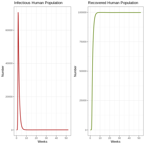
Discussion
Reflection: What can you see in the graph? Look closely at the Y-axis. What proportion of humans are infectious at the same time?
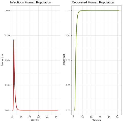
To make this clearer we can create graphs of the proportions:
R
# Review the first epidemic with proportions
p1e <- ggplot(data = out, aes(y = Ih/(Sh+Ih+Rh), x = weeks)) +
  geom_line(color='firebrick', linewidth=1) +
  labs(title = "Infectious Human Population", x = "Weeks", y = "Proportion") +
  theme_bw() +
  coord_cartesian(ylim = c(0,1)) # graph of infectious human population

p2e <- ggplot(data = out, aes(y = Rh/(Sh+Ih+Rh), x = weeks)) +
  geom_line(color='olivedrab', linewidth=1)+
  labs(title = 'Recovered Human Population', x= "Weeks", y= "Proportion") +
  theme_bw() +
  coord_cartesian(ylim = c(0,1)) # graph of recovered human population}

plot_grid(p1e, p2e) # comparison graph of the infectious human population and recovered human population graph
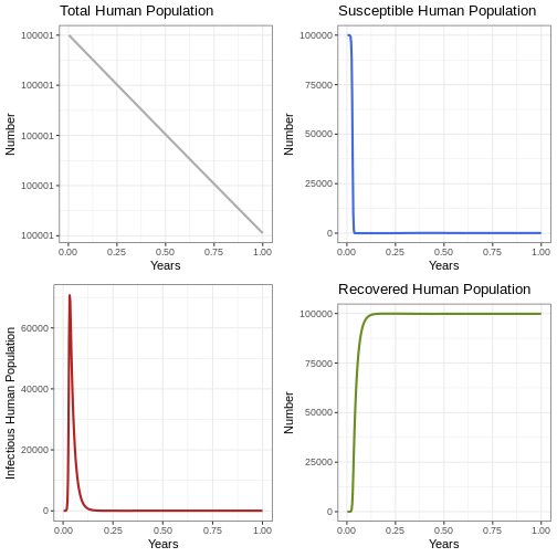
General behaviour (Human population)
Having observed the first epidemic, it is now time to project the epidemic to a longer time frame.
Instruction: Go back to the parameters and change the TIME parameter to 100 years. Run the following code block and observe how many outbreaks occur in the human population and the size of each outbreak.
R
 # Examine the behavior of the model for 100 years
p1h <- ggplot(data = out, aes(y = (Rh + Ih + Sh), x = years)) +
  geom_line(color='grey68', linewidth=1) +
  labs(title = 'Total Human Population', x = "Years", y = "Number") +
  theme_bw()
p2h <- ggplot(data = out, aes(y = Sh, x = years)) +
  geom_line(color='royalblue', linewidth=1)+
  labs(title = 'Susceptible Human Population', x = "Years", y = "Number") +
  theme_bw()
p3h <- ggplot(data = out, aes(y = Ih, x = years)) +
  geom_line(color='firebrick', linewidth=1) +
  labs(y = 'Infectious Human Population', x = "Years", y = "Number") +
  theme_bw()
p4h <- ggplot(data = out, aes(y = Rh, x = years)) +
  geom_line(color='olivedrab', linewidth=1)+
  labs(title = 'Recovered Human Population' , x = "Years", y = "Number") +
  theme_bw()


plot_grid(p1h, p2h, p3h, p4h, ncol = 2)
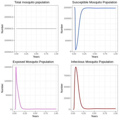
General Behaviour (Mosquito Population)
Instruction: Run the following code block and observe how many outbreaks occur in the mosquito population and the size of each outbreak. Compare the graphs with the human population graphs.
R
# Examine the behavior of the model
p1v <- ggplot(data = out, aes(y = (Sv + Ev + Iv), x = years)) +
  geom_line(color='grey68', linewidth=1) +
  labs(title = 'Total mosquito population', x = "Years", y = "Number")+
  theme_bw()
p2v <- ggplot(data = out, aes(y = Sv, x = years)) +
  geom_line(color='royalblue', linewidth=1) +
  labs(title = 'Susceptible Mosquito Population', x = "Years", y = "Number") +
  theme_bw()
p3v <- ggplot(data = out, aes(y = Ev, x = years)) +
  geom_line(color='orchid', linewidth=1) +
  labs(title = 'Exposed Mosquito Population', x = "Years", y = "Number") +
  theme_bw()
p4v <- ggplot(data = out, aes(y = Iv, x = years)) +
  geom_line(color='firebrick', linewidth=1) +
  labs(title = 'Infectious Mosquito Population', x = "Years", y = "Number") +
  theme_bw()


plot_grid(p1v, p2v, p3v, p4v, ncol = 2)
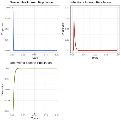
Proportion
Instruction: Run the following code block and compare it to the graphs generated for the human population.
R
#Proportions
p1 <- ggplot(data = out, aes(y = Sh/(Sh+Ih+Rh), x = years)) +
  geom_line(color='royalblue', linewidth=1)+
  ggtitle('Susceptible human population') +
  labs(title = "Susceptible Human Population", x = "Years", y = "Proportion") +
  theme_bw() +
  coord_cartesian(ylim = c(0, 1))
p2 <- ggplot(data = out, aes(y = Ih/(Sh+Ih+Rh), x = years)) +
  geom_line(color='firebrick', linewidth=1) +
  labs(title = "Infectious Human Population", x = "Years", y = "Proportion") +
  theme_bw() +
  coord_cartesian(ylim = c(0, 1))
p3 <- ggplot(data = out, aes(y = Rh/(Sh+Ih+Rh), x = years)) +
  geom_line(color='olivedrab', linewidth=1) +
  labs(title = "Recovered Human Population", x = "Years", y = "Proportion") +
  theme_bw() +
  coord_cartesian(ylim = c(0, 1))


plot_grid(p1, p2, p3, ncol = 2)
Key Points
Check if you have acquired these competences by the end of this lesson:
Recognize how a simple deterministic model is built using ordinary differential equations.
Identify relevant parameters for modeling vector-borne disease (VBD) epidemics.
Learn how to create a diagram for a compartmental model
Translate mathematical equations for a deterministic model into R code.
Use model simulations to explore transmission scenarios and the potential impact of interventions.
Contributions
- Zulma Cucunuba & Pierre Nouvellet: Initial version
- Kelly Charinga & Zhian N. Kamvar: Editing
- José M. Velasco-Spain: Translation from English to Spanish and Editing
- Andree Valle-Campos: Minor Editions
References
de Carvalho, S. S., Rodovalho, C. M., Gaviraghi, A., Mota, M. B. S., Jablonka, W., Rocha-Santos, C., Nunes, R. D., Sá-Guimarães, T. da E., Oliveira, D. S., Melo, A. C. A., Moreira, M. F., Fampa, P., Oliveira, M. F., da Silva-Neto, M. A. C., Mesquita, R. D., & Atella, G. C. (2021). Aedes aegypti post-emergence transcriptome: Unveiling the molecular basis for the hematophagic and gonotrophic capacitation. PLoS Neglected Tropical Diseases, 15(1), 1–32. https://doi.org/10.1371/journal.pntd.0008915
Chang, C., Ortiz, K., Ansari, A., & Gershwin, M. E. (2016). The Zika outbreak of the 21st century. Journal of Autoimmunity, 68, 1–13. https://doi.org/10.1016/j.jaut.2016.02.006
Cori, A., Ferguson, N. M., Fraser, C., & Cauchemez, S. (2013). A new framework and software to estimate time-varying reproduction numbers. during epidemics. American Journal of Epidemiology, 178(9), 1505–1512. https://doi.org/10.1093/aje/kwt133
Duffy, M. R., Chen, T.-H., Hancock, W. T., Powers, A. M., Kool, J. L., Lanciotti, R. S., Pretrick, M., Marfel, M., Holzbauer, S., Dubray, C., Guillaumot, L., Griggs, A., Bel, M., Lambert, A. J., Laven, J., Kosoy, O., Panella, A., Biggerstaff, B. J., Fischer, M., & Hayes, E. B. (2009). Zika Virus Outbreak on Yap Island, Federated States of Micronesia. New New England Journal of Medicine, 360(24), 2536–2543. https://doi.org/10.1056/nejmoa0805715
Ferguson, N. M., Cucunubá, Z. M., Dorigatti, I., Nedjati-Gilani, G. L., Donnelly, C. A., Basáñez, M. G., Nouvellet, P., & Lessler, J. (2016). Countering the Zika epidemic in Latin America. Science, 353(6297). https://doi.org/10.1126/science.aag0219
Heesterbeek, J. A. P. (2002). A brief history of R0 and a recipe for its calculation. Acta Biotheoretica, 50(3). https://doi.org/10.1023/A:1016599411804
Lee, E. K., Liu, Y., & Pietz, F. H. (2016). A Compartmental Model for Zika Virus with Dynamic Human and Vector Populations. AMIA … Annual Symposium Proceedings. AMIA Symposium, 2016, 743–752.
Pettersson, J. H. O., Eldholm, V., Seligman, S. J., Lundkvist, Å., Falconar, A. K., Gaunt, M. W., Musso, D., Nougairède, A., Charrel, R., Gould, E. A., & de Lamballerie, X. (2016). How did zika virus emerge in the Pacific Islands and Latin America? MBio, 7(5). https://doi.org/10.1128/mBio.01239-16