Estimate R and relative susceptibility from age-stratified pre- and post-epidemic serological data

What do we have?

• Serological data measuring rise in influenza titres during the 2009 A/H1N1p pandemic in different age groups (i.e. proxy for infection)
• Social mixing data from socialmixr

Steps in code

# Load required packages
library(finalsize)
library(socialmixr)
library(MCMCpack)
library(readr)
library(dplyr)
library(ggplot2)

# Load serological data
# source:
# Kwok KO, Cowling BJ, Wei VW, Wu KM, Read JM, Lessler J, Cummings DA, Peiris JS, Riley S. 
# Social contacts and the locations in which they occur as risk factors for influenza infection. 
# Proc Biol Sci. 2014 Aug 22;281(1789):20140709. doi: 10.1098/rspb.2014.0709. 
# PMID: 25009062; PMCID: PMC4100506.
# https://pmc.ncbi.nlm.nih.gov/articles/instance/4100506/
hk_serology <- readr::read_csv("https://github.com/epiverse-trace/howto/raw/refs/heads/main/data/rspb20140709supp2.csv")

# Allocate ages to bands
age_limits <- c(3,18,25,40,65)
age_group <- sapply(hk_serology$age,function(x){sum(x>=age_limits)})
hk_serology$age_group <- age_group

# Load HK social mixing data
contact_data <- socialmixr::contact_matrix(
  polymod,
  countries = "United Kingdom",
  age.limits = age_limits,
  symmetric = TRUE
)

demography_vector <- contact_data$demography$population

# Define model
model_function <- function(param){
  r0 <- param[1]
  alpha_val <- param[2]
  
  contact_matrix = t(contact_data$matrix)
  contact_matrix = contact_matrix / max(eigen(contact_matrix)$values)
  
  names(demography_vector) = contact_data$demography$age.group
  n_demo_grps = length(demography_vector)
  
  contact_matrix = contact_matrix / demography_vector
  
  susceptibility = matrix(
    data = c(1, alpha_val*rep(1,n_demo_grps-1)),
    n_demo_grps
  )
  
  n_risk_grps = 1L
  p_susceptibility = matrix(1, n_demo_grps, n_risk_grps)
  
  simulation_output <- finalsize::final_size(
    r0 = r0,
    contact_matrix = contact_matrix,
    demography_vector = demography_vector,
    susceptibility = susceptibility,
    p_susceptibility = p_susceptibility,
    solver = "iterative"
  )
  
  return(simulation_output)
}

# Define likelihood function
likelihood_function <- function(param,data) {
  # Ensure positive parameters
  if (any(param <= 0)) return(-Inf)

  simulation_output <- model_function(param)
  
  # Assuming non-informative priors for alpha and beta
  log_prior <- 0 # Can refine if have different priors
  
  # Calculate log-likelihood
  test_positive <- hk_serology$ffold
  log_likelihood <- log(
    test_positive*simulation_output$p_infected[hk_serology$age_group] + 
      (1-test_positive)*(1-simulation_output$p_infected[hk_serology$age_group])
  )
  log_likelihood_total <- sum(log_likelihood)
  
  # Check for valid output
  if(is.na(log_likelihood_total)){
    log_likelihood_total <- -Inf
  }
  
  # Return log-posterior (log-likelihood + log-prior)
  return(log_likelihood_total + log_prior)
}

## Set up MCMCpack for Monte Carlo estimation
initial_param <- c(r0=1.5, alpha=0.8) # Initial guess for shape and rate

n_mcmc <- 1000

output <- MCMCpack::MCMCmetrop1R(
  fun = likelihood_function, 
  theta.init = initial_param,
  mcmc = n_mcmc, # Number of MCMC iterations
  burnin = 100, # Burn-in period
  verbose = FALSE, # Turn off verbose output
  data = hk_serology
)
#> 
#> 
#> @@@@@@@@@@@@@@@@@@@@@@@@@@@@@@@@@@@@@@@@@@@@@@@@@@@@@@@@@
#> The Metropolis acceptance rate was 0.55091
#> @@@@@@@@@@@@@@@@@@@@@@@@@@@@@@@@@@@@@@@@@@@@@@@@@@@@@@@@@

# Plot outputs
data_summary <- stats::aggregate(
  x = ffold ~ age_group,
  data = hk_serology, 
  FUN = function(x){mean(x == 1)}
)

sample_outputs <- output[sample(1:n_mcmc,10),]
sample_simulate <- apply(sample_outputs,1,model_function)

# Combine all list elements into a single data frame
combined_data <- do.call(rbind, lapply(1:length(sample_simulate), function(i) {
  cbind(sample_simulate[[i]], Simulation = i)
}))

combined_data$age_index <- base::match(
  x = combined_data$demo_grp,
  table = contact_data$demography$age.group
)

# Calculate mean and standard deviation of p_infected for each demo_grp
summary_data <- combined_data %>%
  dplyr::group_by(age_index) %>%
  dplyr::summarise(
    Mean_p_infected = mean(p_infected),
    SD_p_infected = sd(p_infected)
  ) %>%
  dplyr::ungroup()

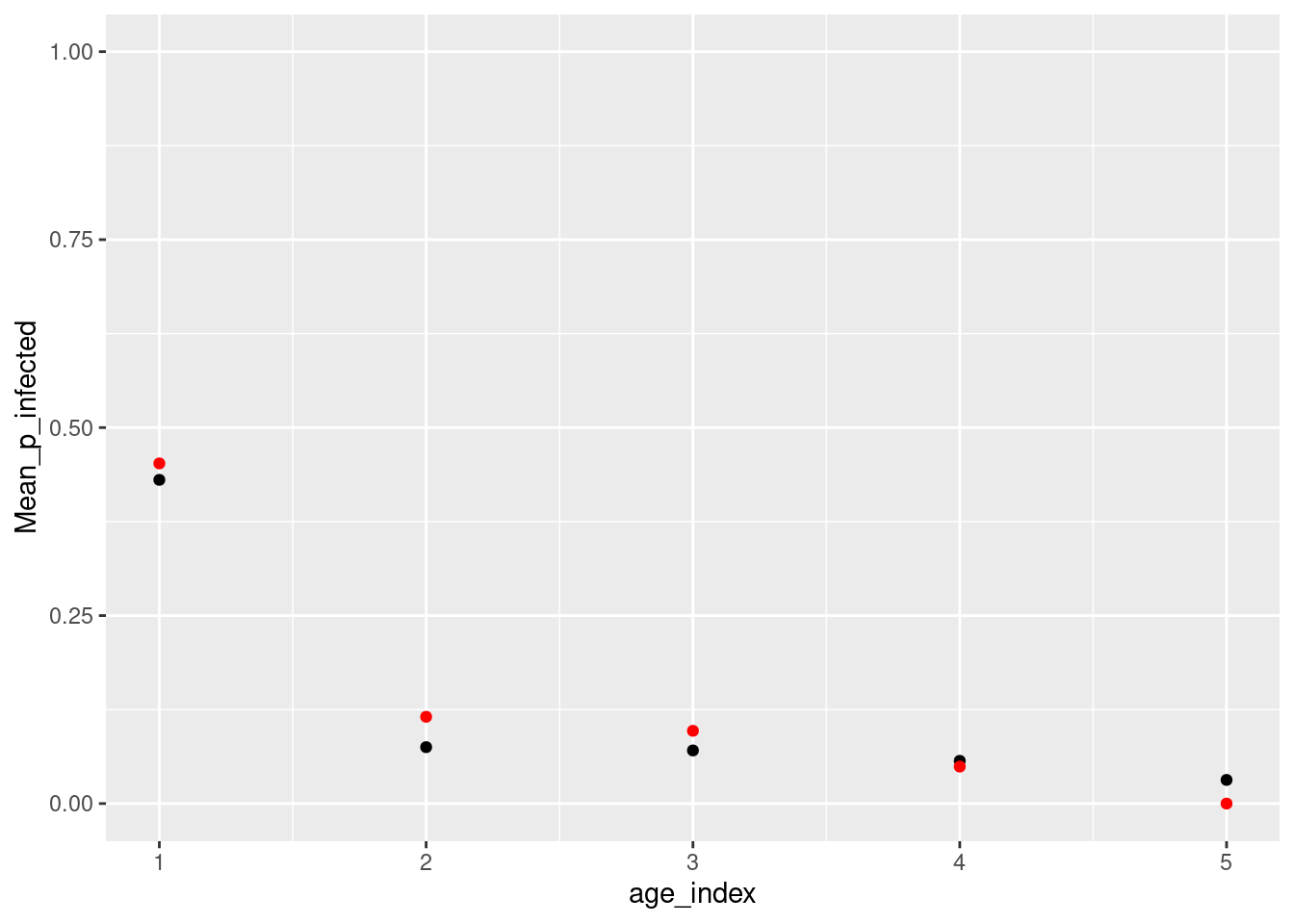
# Plotting
summary_data %>% 
  dplyr::left_join(data_summary, by = c("age_index" = "age_group")) %>% 
  ggplot() +
  geom_point(aes(x = age_index, y = Mean_p_infected)) +
  geom_point(aes(x = age_index, y = ffold),pch=19,col="red") +
  ylim(0,1)

Steps in detail

• Want to estimate the reproduction number and relative susceptibility in older age groups from the pattern of infection, based on the final epidemic size in an age-stratified SIR-like model, following the methods of Kucharski et al (2014) and using Markov chain Monte Carlo.
• We use serological data from the 2009 pandemic in Hong Kong in Kwok et al (2009), and social mixing data from POLYMOD in the UK as an assumed contact matrix using socialmixr.
• We define the likelihood of observing a given serological pattern by simulating age-specific final epidemic size using the finalsize package.
• We use {MCMCpack} to estimate the parameters using MCMC.
• Finally, we plot the observed outputs against the model fits.