Estimate Effective Reproduction Number (Rt) from Weekly Reported Confirmed Cases

Author

James M. Azam

Published

July 31, 2025

What do we have?

Week aggregate of new COVID confirmed cases
Serial interval stored in epiparameter
Incubation period stored in epiparameter

Steps in code

Using `{EpiNow2}`

# ============================================================================== #
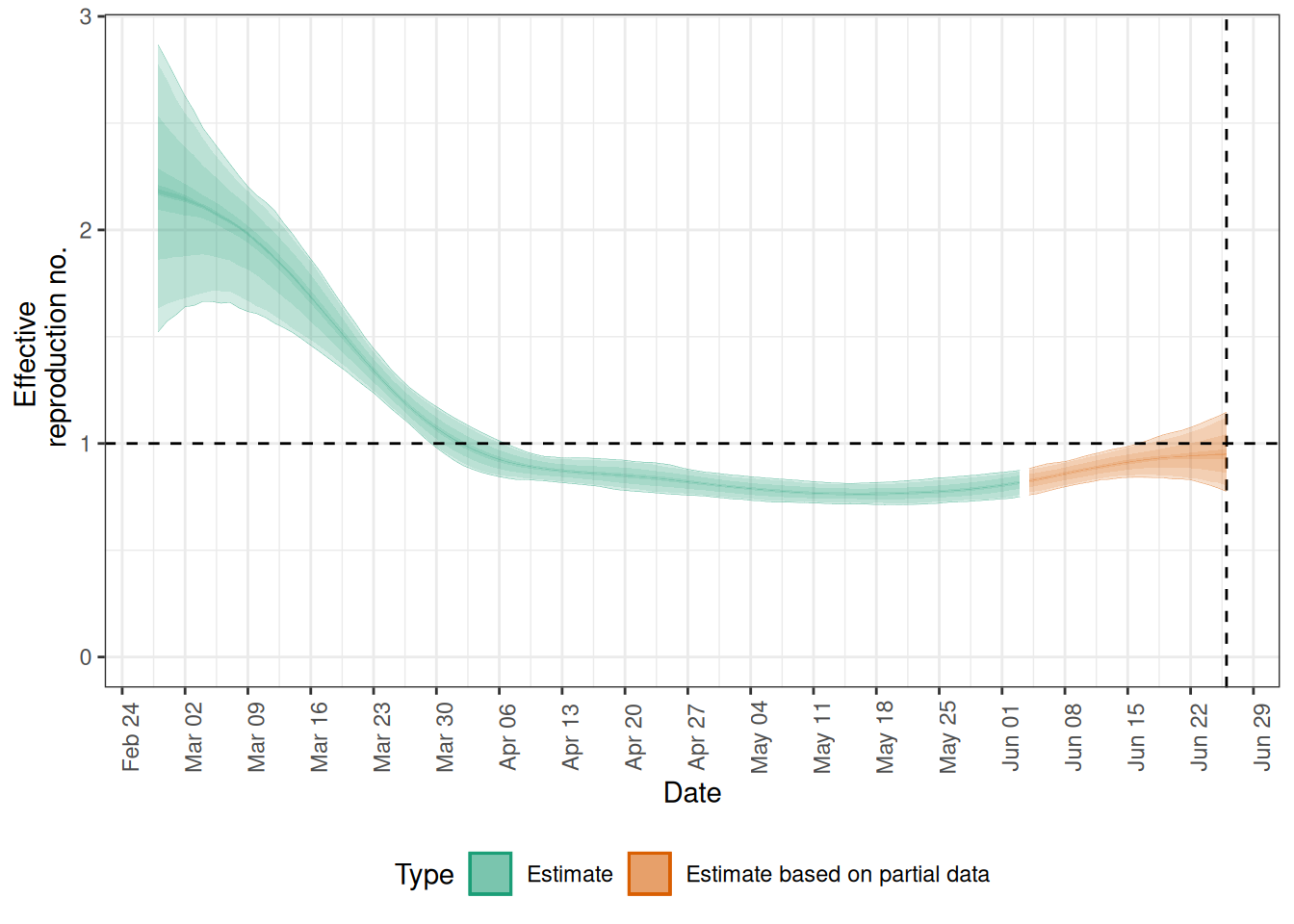
# SETUP AND DATA PREPARATION
# ============================================================================== #

# Load necessary packages for analysis
library(EpiNow2) # To estimate time-varying reproduction number
library(epiparameter) # To extract epidemiological parameters
library(data.table) # For data manipulation
library(parallel) # For parallel processing
library(withr) # For setting local options
library(dplyr) # For data manipulation
library(ggplot2) # For data visualisation
library(janitor) # For data cleaning

# Set the number of cores for faster processing
withr::local_options(list(mc.cores = parallel::detectCores() - 1))

# Use the example data for confirmed cases from EpiNow2
reported_cases <- EpiNow2::example_confirmed
reported_cases_weekly <- data.table::copy(reported_cases)

# Aggregate the daily cases to weekly cases (sum of daily cases)
reported_cases_weekly[, confirm := frollsum(confirm, 7)]
reported_cases_weekly <- reported_cases_weekly[seq(7, nrow(reported_cases_weekly), 7)]

# Create data with missing dates filled in for EpiNow2
input_data_epinow <- EpiNow2::fill_missing(
  reported_cases_weekly,
  missing_dates = "accumulate",
  initial_accumulate = 1 # Don't model the first data point (to match EpiEstim method)
)

# ============================================================================== #
# DEFINE EPIDEMIOLOGICAL PARAMETERS AND DISTRIBUTIONS
# ============================================================================== #

# Extract distribution the incubation period for COVID-19
covid_incubation_dist <- epiparameter::epiparameter_db(
  disease = "covid",
  epi_name = "incubation",
  single_epiparameter = TRUE
)

# Extract the serial interval distribution
serial_interval_dist <- epiparameter::epiparameter_db(
  disease = "covid",
  epi_name = "serial",
  single_epiparameter = TRUE
)

# ============================================================================== #
# ESTIMATE INFECTIONS AND Rt WITH EPINOW2
# ============================================================================== #

# Extract parameters and maximum of the distribution for EpiNow2
incubation_params <- epiparameter::get_parameters(covid_incubation_dist)
incubation_max_days <- round(quantile(covid_incubation_dist, 0.999)) # Upper 99.9% range needed for EpiNow2

# Create a LogNormal object for the incubation period
incubation_lognormal <- EpiNow2::LogNormal(
  meanlog = incubation_params[["meanlog"]],
  sdlog = incubation_params[["sdlog"]],
  max = incubation_max_days
)

# Extract parameters and maximum of the distribution for EpiNow2
serial_interval_params <- epiparameter::get_parameters(serial_interval_dist)
serial_interval_max_days <- round(quantile(serial_interval_dist, 0.999)) # Upper 99.9% range needed for EpiNow2

# Create a LogNormal object for the serial interval
serial_interval_lognormal <- EpiNow2::LogNormal(
  meanlog = serial_interval_params[["meanlog"]],
  sdlog = serial_interval_params[["sdlog"]],
  max = serial_interval_max_days
)

# Estimate infections using EpiNow2
estimates_epinow <- EpiNow2::epinow(
  data = input_data_epinow,
  generation_time = generation_time_opts(serial_interval_lognormal),
  forecast = forecast_opts(horizon = 0, accumulate = 1), # Forecasting is turned off to match with EpiEstim
  rt = rt_opts(
    prior = Gamma(mean = 5, sd = 5) # same prior as used in EpiEstim default
  ),
  CrIs = c(0.025, 0.05, 0.25, 0.75, 0.95, 0.975), # same prior as used in EpiEstim default
  stan = EpiNow2::stan_opts(samples = 1000, chains = 2), # revert to 4 chains for better inference
  verbose = FALSE
)
#> WARN [2025-07-31 16:57:04] epinow: There were 34 divergent transitions after warmup. See
#> https://mc-stan.org/misc/warnings.html#divergent-transitions-after-warmup
#> to find out why this is a problem and how to eliminate them. - 
#> WARN [2025-07-31 16:57:04] epinow: Examine the pairs() plot to diagnose sampling problems
#>  - 
#> WARN [2025-07-31 16:57:05] epinow: Bulk Effective Samples Size (ESS) is too low, indicating posterior means and medians may be unreliable.
#> Running the chains for more iterations may help. See
#> https://mc-stan.org/misc/warnings.html#bulk-ess -

# Initial look at the output
plot(estimates_epinow$plots$R)

Using `{EpiEstim}`

The EpiEstim example follows the methodology outlined in the EpiEstim vignette in https://mrc-ide.github.io/EpiEstim/articles/EpiEstim_aggregated_data.html.

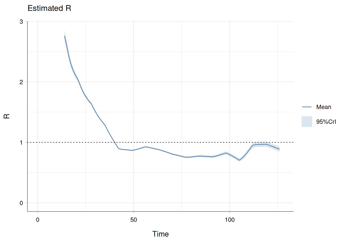
# Load necessary packages for analysis
library(EpiEstim) # To estimate time-varying reproduction number

# ============================================================================== #
# ESTIMATE RT WITH EPIESTIM
# ============================================================================== #

# Prepare serial interval distribution. We'll reuse the serial interval distribution
# extracted earlier.
si_mean <- serial_interval_dist$summary_stats$mean
si_sd <- serial_interval_dist$summary_stats$sd

# Prepare the input data
input_data_epiestim <- reported_cases_weekly %>%
  dplyr::rename(I = confirm) %>%
  dplyr::mutate(
    dates = as.Date(date),
    I = as.integer(I)
  ) %>%
  dplyr::select(I)

# Estimate Rt using weekly aggregated data
estimates_epiestim <- EpiEstim::estimate_R(
  incid = input_data_epiestim$I,
  dt = 7L, # Aggregation window
  dt_out = 7L, # Estimation rolling window
  recon_opt = "naive",
  method = "parametric_si",
  config = make_config(
    list(mean_si = si_mean, std_si = si_sd)
  )
)

# Initial look at the output
plot(estimates_epiestim, "R") # Rt estimates only

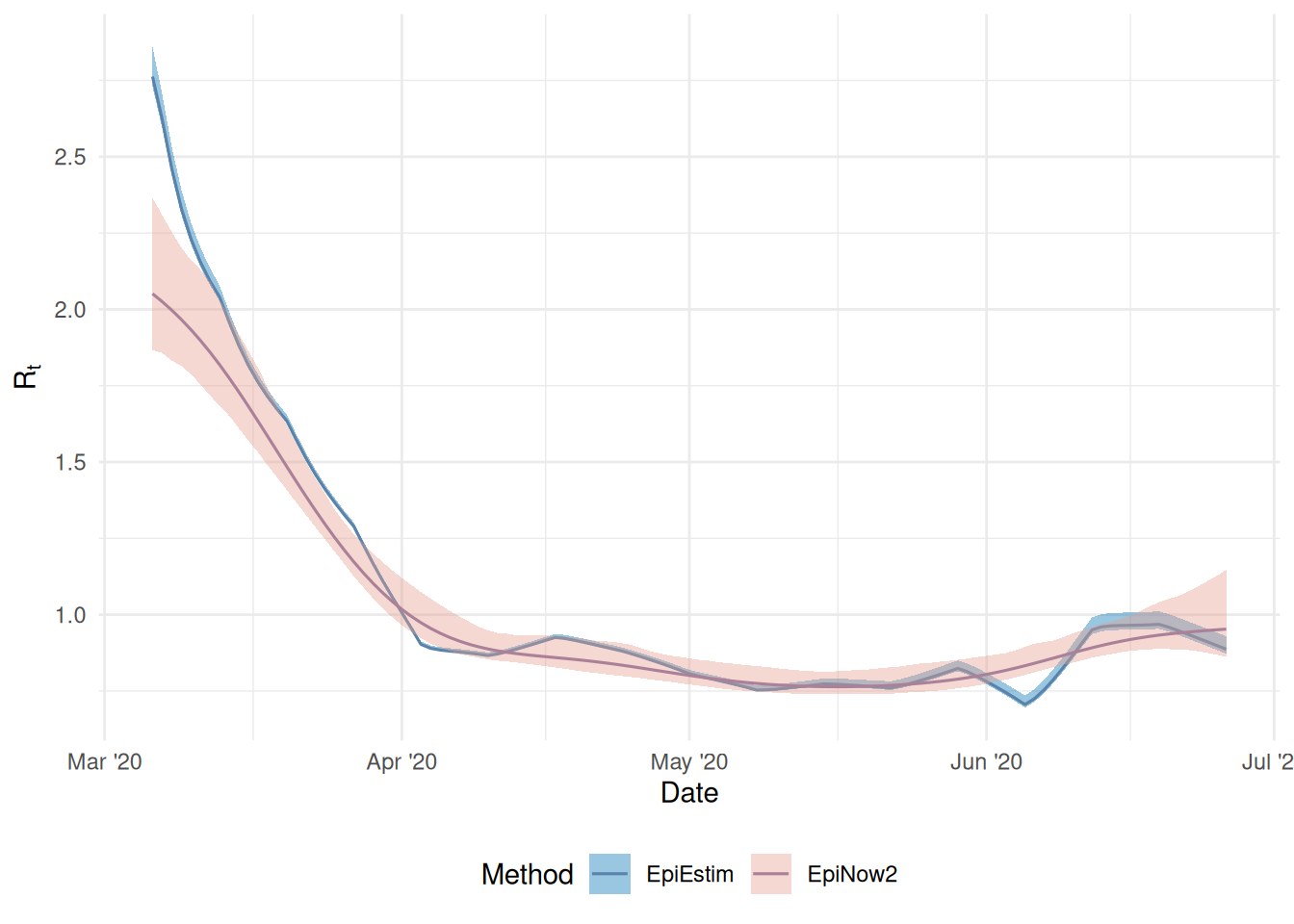
Compare `{EpiNow2}` and `{EpiEstim}`

# ==============================================================================
# COMPARING THE RESULTS FROM EpiNow2 and EpiEstim
# ==============================================================================
# Extract and process the Rt estimates from EpiEstim output
epiestim_Rt <- estimates_epiestim$R %>%
  dplyr::mutate(method = "EpiEstim")

# Align the Rt estimates with the original dates in the complete time series
complete_dates <- seq(
  min(reported_cases_weekly$date),
  max(reported_cases_weekly$date),
  1
)

Rt_ts_epiestim <- data.frame(date = complete_dates) %>%
  dplyr::mutate(lookup = seq_along(complete_dates)) %>%
  dplyr::inner_join(
    epiestim_Rt,
    by = join_by(lookup == t_start)
  ) %>%
  dplyr::select(-c(lookup)) %>%
  janitor::clean_names()

# Extract and process the Rt estimates from EpiNow2 output
Rt_ts_epinow <- estimates_epinow$estimates$summarised %>%
  dplyr::filter(variable == "R") %>%
  dplyr::filter(date >= min(Rt_ts_epiestim$date, na.rm = TRUE)) %>% # Start from EpiEstim's first estimate
  dplyr::mutate(method = "EpiNow2") %>%
  janitor::clean_names()

# Plot the results
rt_plot <- ggplot() +
  # EpiEstim Ribbon
  geom_ribbon(
    data = Rt_ts_epiestim,
    aes(
      x = date,
      ymin = quantile_0_25_r,
      ymax = quantile_0_975_r,
      fill = method
    ),
    alpha = 0.4
  ) +
  # EpiEstim Line
  geom_line(
    data = Rt_ts_epiestim,
    aes(
      x = date,
      y = mean_r,
      color = method
    ),
    linewidth = 0.55
  ) +
  # EpiNow2 Ribbon
  geom_ribbon(
    data = Rt_ts_epinow,
    aes(
      x = date,
      ymin = lower_75,
      ymax = upper_97_5,
      fill = method
    ),
    alpha = 0.4
  ) +
  # EpiNow2 Line
  geom_line(
    data = Rt_ts_epinow,
    aes(
      x = date,
      y = mean,
      color = method
    ),
    linewidth = 0.55
  ) +
  labs(
    x = "Date",
    y = expression(R[t]),
    color = "Method",
    fill = "Method"
  ) +
  scale_fill_manual(
    values = c(
      "EpiNow2" = "#E69E90",
      "EpiEstim" = "#0072B2"
    )
  ) +
  scale_color_manual(
    values = c(
      "EpiNow2" = "#AB8199",
      "EpiEstim" = "#5983AB"
    )
  ) +
  scale_x_date(date_breaks = "month", date_labels = "%b '%y") +
  theme_minimal() +
  theme(legend.position = "bottom")

plot(rt_plot)

Steps in detail

tidyverse package is loaded to manage data frame objects.

Please note that the code assumes the necessary packages are already installed. If they are not, you can install them using first the install.packages("pak") function and then the pak::pak() function for both packages in CRAN or GitHub before loading them with library().

Additionally, make sure to adjust the serial interval distribution parameters according to the specific outbreak you are analyzing.

What do we have?

Steps in code

Using {EpiNow2}

Using {EpiEstim}

Compare {EpiNow2} and {EpiEstim}

Steps in detail

Related

Using `{EpiNow2}`

Using `{EpiEstim}`

Compare `{EpiNow2}` and `{EpiEstim}`