Reconstruct infection dynamics from incidence data on delayed outcomes like deaths

What do we have?

• Time series of new outcomes (e.g. deaths) per day.
• Estimates of the delay from infection-to-onset and onset-to-death distributions

Steps in code

Example 1

Reconstruct SARS-CoV-2 infection dynamics in the UK from daily data on deaths, 2020

# Load required packages
library(incidence2) # for uk covid daily deaths
library(EpiNow2) # to estimate time-varying reproduction number
library(epiparameter) # to access delay distributions
library(cfr) # for Ebola data (included in this package)
library(dplyr) # to format input and outputs
library(ggplot2) # to generate plots

# Set number of cores
withr::local_options(list(mc.cores = 4))

# Extract data on UK COVID deaths and format for EpiNow2
incidence_data <- incidence2::covidregionaldataUK %>% 
  # preprocess missing values
  tidyr::replace_na(list(deaths_new = 0)) %>%
  # compute the daily incidence
  incidence2::incidence(
    date_index = "date",
    counts = "deaths_new",
    count_values_to = "confirm",
    date_names_to = "date",
    complete_dates = TRUE
  ) %>%
  dplyr::select(-count_variable) %>% 
  # Focus on early 2020 period and sort by ascending date
  dplyr::filter(date<"2020-07-01" & date>="2020-03-01") %>% 
  # convert to tibble format for simpler data frame output
  dplyr::as_tibble()

# Preview data
incidence_data
#> # A tibble: 122 × 2
#>    date       confirm
#>    <date>       <dbl>
#>  1 2020-03-01       0
#>  2 2020-03-02       2
#>  3 2020-03-03       4
#>  4 2020-03-04       0
#>  5 2020-03-05       5
#>  6 2020-03-06       0
#>  7 2020-03-07       0
#>  8 2020-03-08       6
#>  9 2020-03-09      10
#> 10 2020-03-10       6
#> # ℹ 112 more rows

# Define parameters
# Extract infection-to-death distribution (from Aloon et al)
incubation_period_in <-
  epiparameter::epiparameter_db(
    disease = "covid",
    epi_name = "incubation",
    single_epiparameter = TRUE
  )

# Summarise distribution and type
print(incubation_period_in)
#> Disease: COVID-19
#> Pathogen: SARS-CoV-2
#> Epi Parameter: incubation period
#> Study: Linton N, Kobayashi T, Yang Y, Hayashi K, Akhmetzhanov A, Jung S, Yuan
#> B, Kinoshita R, Nishiura H (2020). "Incubation Period and Other
#> Epidemiological Characteristics of 2019 Novel Coronavirus Infections
#> with Right Truncation: A Statistical Analysis of Publicly Available
#> Case Data." _Journal of Clinical Medicine_. doi:10.3390/jcm9020538
#> <https://doi.org/10.3390/jcm9020538>.
#> Distribution: lnorm (days)
#> Parameters:
#>   meanlog: 1.525
#>   sdlog: 0.629

# Get parameters and format for EpiNow2 using LogNormal input
incubation_params <- epiparameter::get_parameters(incubation_period_in)

# Find the upper 99.9% range by the interval
incubation_max <- round(quantile(incubation_period_in,0.999))

incubation_period <- EpiNow2::LogNormal(
  meanlog = incubation_params[["meanlog"]], 
  sdlog = incubation_params[["sdlog"]], 
  max = incubation_max
)

## Set onset to death period (from Linton et al)
onset_to_death_period_in <-
  epiparameter::epiparameter_db(
    disease = "covid",
    epi_name = "onset to death",
    single_epiparameter = TRUE
  )

# Summarise distribution and type
print(onset_to_death_period_in)
#> Disease: COVID-19
#> Pathogen: SARS-CoV-2
#> Epi Parameter: onset to death
#> Study: Linton N, Kobayashi T, Yang Y, Hayashi K, Akhmetzhanov A, Jung S, Yuan
#> B, Kinoshita R, Nishiura H (2020). "Incubation Period and Other
#> Epidemiological Characteristics of 2019 Novel Coronavirus Infections
#> with Right Truncation: A Statistical Analysis of Publicly Available
#> Case Data." _Journal of Clinical Medicine_. doi:10.3390/jcm9020538
#> <https://doi.org/10.3390/jcm9020538>.
#> Distribution: lnorm (days)
#> Parameters:
#>   meanlog: 2.863
#>   sdlog: 0.534

# Get parameters and format for EpiNow2 using LogNormal input
onset_to_death_params <- epiparameter::get_parameters(onset_to_death_period_in)

# Find the upper 99.9% range by the interval
onset_to_death_max <- round(quantile(onset_to_death_period_in,0.999))

onset_to_death_period <- LogNormal(
  meanlog = onset_to_death_params[["meanlog"]], 
  sdlog = onset_to_death_params[["sdlog"]], 
  max = onset_to_death_max
)

## Combine infection-to-onset and onset-to-death
infection_to_death <- incubation_period + onset_to_death_period

# Plot underlying delay distributions
# plot(infection_to_death)

# Extract serial interval distribution distribution (from Yang et al)
serial_interval_in <-
  epiparameter::epiparameter_db(
    disease = "covid",
    epi_name = "serial",
    single_epiparameter = TRUE
  )

# Summarise distribution and type
print(serial_interval_in)
#> Disease: COVID-19
#> Pathogen: SARS-CoV-2
#> Epi Parameter: serial interval
#> Study: Nishiura H, Linton N, Akhmetzhanov A (2020). "Serial interval of novel
#> coronavirus (COVID-19) infections." _International Journal of
#> Infectious Diseases_. doi:10.1016/j.ijid.2020.02.060
#> <https://doi.org/10.1016/j.ijid.2020.02.060>.
#> Distribution: lnorm (days)
#> Parameters:
#>   meanlog: 1.386
#>   sdlog: 0.568

# Discretise serial interval for input into EpiNow2
serial_int_discrete <- epiparameter::discretise(serial_interval_in)

# Find the upper 99.9% range by the interval
serial_int_discrete_max <- quantile(serial_int_discrete,0.999)

# Get parameters
serial_params <- epiparameter::get_parameters(serial_int_discrete)

# Define parameters using LogNormal input
serial_interval_covid <- LogNormal(
  meanlog = serial_params[["meanlog"]],
  sdlog = serial_params[["sdlog"]],
  max = serial_int_discrete_max
)
# Run infection estimation model
epinow_estimates <- epinow(
  data = incidence_data, # time series data
  # assume generation time = serial interval
  generation_time = generation_time_opts(serial_interval_covid),
  # delay from infection-to-death
  delays = delay_opts(infection_to_death),
  # no Rt estimation
  rt = NULL,
  # change default Gaussian Process priors
  gp = gp_opts(alpha = Normal(0, 0.05))
)

# Extract infection estimates from the model output
infection_estimates <- epinow_estimates$estimates$summarised %>% 
  dplyr::filter(variable=="infections")

# Plot output
epinow_estimates$plots$infections +
  geom_vline(aes(xintercept = as.Date("2020-03-16")), linetype = 3) +
  geom_text(aes(x = as.Date("2020-03-16"), 
                y = 3000,
                label = "Non-essential contact advice"),
            hjust = 0) +
  geom_vline(aes(xintercept = as.Date("2020-03-23")), linetype = 3) +
  geom_text(aes(x = as.Date("2020-03-23"), 
                y = 2500,
                label = "Stay-at-home order (i.e. lockdown)"),
            hjust = 0) +
  labs(
    title = "Estimated dynamics of SARS-CoV-2 infections
    among those with subsequent fatal outcomes in the UK,
    reconstructed using data on reported deaths.",
    subtitle = "Dashed lines show dates of
    UK non-essential contact advice (16 Mar)
    and lockdown (23 Mar)."
  )

Example 2

Reconstruct Ebola infection dynamics in Zaire from data on cases, 1976

# Load required packages
library(incidence2) # for uk covid daily deaths
library(EpiNow2) # to estimate time-varying reproduction number
library(epiparameter) # to access delay distributions
library(cfr) # for Ebola data (included in this package)
library(dplyr) # to format input and outputs
library(ggplot2) # to generate plots

# Set number of cores
withr::local_options(list(mc.cores = 4))

# Load Ebola data from the CFR package
data("ebola1976")

# Extract data on case onsets and format for EpiNow2
incidence_data_ebola <- ebola1976 %>%
  dplyr::as_tibble() %>% # for simpler dataframe output
  dplyr::select(date,cases) %>%
  dplyr::rename(confirm = cases) %>%
  dplyr::filter(date >= "1976-09-01")

# Preview data
incidence_data_ebola
#> # A tibble: 66 × 2
#>    date       confirm
#>    <date>       <int>
#>  1 1976-09-01       1
#>  2 1976-09-02       1
#>  3 1976-09-03       1
#>  4 1976-09-04       4
#>  5 1976-09-05       1
#>  6 1976-09-06       1
#>  7 1976-09-07       3
#>  8 1976-09-08       2
#>  9 1976-09-09       7
#> 10 1976-09-10       9
#> # ℹ 56 more rows

# Extract infection-to-death distribution (from WHO Ebola Response Team)
incubation_period_ebola_in <-
  epiparameter::epiparameter_db(
    disease = "ebola",
    epi_name = "incubation",
    single_epiparameter = TRUE
  )

# Summarise distribution and type
print(incubation_period_ebola_in)
#> Disease: Ebola Virus Disease
#> Pathogen: Ebola Virus
#> Epi Parameter: incubation period
#> Study: WHO Ebola Response Team, Agua-Agum J, Ariyarajah A, Aylward B, Blake I,
#> Brennan R, Cori A, Donnelly C, Dorigatti I, Dye C, Eckmanns T, Ferguson
#> N, Formenty P, Fraser C, Garcia E, Garske T, Hinsley W, Holmes D,
#> Hugonnet S, Iyengar S, Jombart T, Krishnan R, Meijers S, Mills H,
#> Mohamed Y, Nedjati-Gilani G, Newton E, Nouvellet P, Pelletier L,
#> Perkins D, Riley S, Sagrado M, Schnitzler J, Schumacher D, Shah A, Van
#> Kerkhove M, Varsaneux O, Kannangarage N (2015). "West African Ebola
#> Epidemic after One Year — Slowing but Not Yet under Control." _The New
#> England Journal of Medicine_. doi:10.1056/NEJMc1414992
#> <https://doi.org/10.1056/NEJMc1414992>.
#> Distribution: gamma (days)
#> Parameters:
#>   shape: 1.578
#>   scale: 6.528

# Get parameters and format for EpiNow2 using Gamma input
incubation_ebola_params <- epiparameter::get_parameters(incubation_period_ebola_in)

# Find the upper 99.9% range by the interval
incubation_ebola_max <- round(quantile(incubation_period_ebola_in,0.999))

incubation_period_ebola <- EpiNow2::Gamma(
  shape = incubation_ebola_params[["shape"]], 
  rate = 1/incubation_ebola_params[["scale"]], 
  max = incubation_ebola_max
)

# Plot delay distribution
# plot(incubation_period_ebola)

# Extract serial interval distribution distribution
# (from WHO Ebola Response Team)
serial_interval_ebola_in <-
  epiparameter::epiparameter_db(
    disease = "ebola",
    epi_name = "serial",
    single_epiparameter = TRUE
  )

# Summarise distribution and type
# print(serial_interval_ebola_in)

# Discretise serial interval for input into EpiNow2
serial_int_ebola_discrete <- epiparameter::discretise(serial_interval_ebola_in)

# Find the upper 99.9% range by the interval
serial_int_ebola_discrete_max <- quantile(serial_int_ebola_discrete,0.999)

# Define parameters using LogNormal input
serial_ebola_params <- epiparameter::get_parameters(serial_int_ebola_discrete)

serial_interval_ebola <- EpiNow2::Gamma(
  shape = serial_ebola_params[["shape"]],
  rate = 1/serial_ebola_params[["scale"]],
  max = serial_int_ebola_discrete_max
)

# Run infection estimation model
epinow_estimates <- EpiNow2::epinow(
  data = incidence_data_ebola, # time series data
  # assume generation time = serial interval
  generation_time = generation_time_opts(serial_interval_ebola),
  # delay from infection-to-death
  delays = delay_opts(incubation_period_ebola),
  rt = NULL,
  # change default Gaussian Process priors
  gp = gp_opts(alpha = Normal(0, 0.05)),
  # use zero-centered prior
  # instead of one centered around shifted reported cases
  backcalc = backcalc_opts(prior = "none")
)

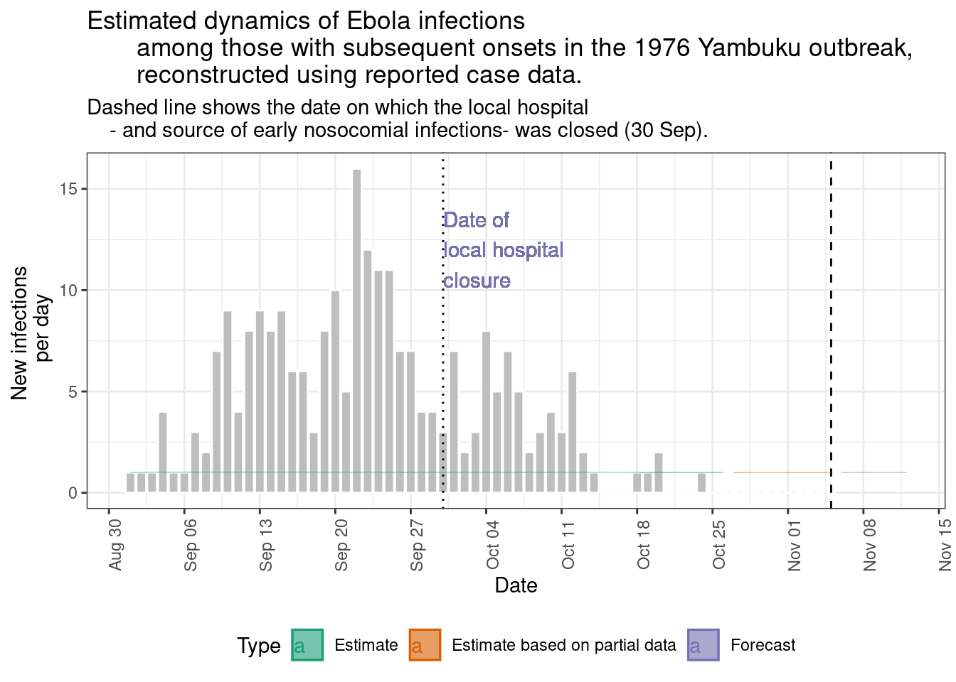
# Extract infection estimates from the model output
infection_estimates <- epinow_estimates$estimates$summarised %>% 
  dplyr::filter(variable=="infections")

# Plot output
epinow_estimates$plots$infections +
  geom_vline(aes(xintercept = as.Date("1976-09-30")), linetype = 3) +
  geom_text(aes(x = as.Date("1976-09-30"), 
                y = 12,
                label = "Date of\nlocal hospital\nclosure"),
            hjust = 0) +
  labs(
    title = "Estimated dynamics of Ebola infections
       among those with subsequent onsets in the 1976 Yambuku outbreak,
       reconstructed using reported case data.",
    subtitle = "Dashed line shows the date on which the local hospital
    - and source of early nosocomial infections- was closed (30 Sep).")

Steps in detail

• We assume new infections each day have a prior based on a Gaussian process, which allows for faster estimation from delayed outcome data than modelling the full transmission process (and hence also estimating the time varying reproduction number \(R_t\)).

Example 1

• Example 1 aims to reconstruct SARS-CoV-2 infection dynamics in the UK from daily data on deaths
• First, we load daily data on reported COVID deaths from the UK COVID dashboard by copying the ‘download data as csv’ link, then using the httr package to import into R and format as a data.frame.
• The EpiNow2 package expects data in a two column format with names date and confirm so we format the imported data accordingly.
• Next, we import an estimate of the COVID incubation period (i.e. delay from infection to symptom onset) and onset-to-death distributions from epiparameter, then combine these two distributions to specify the infection-to-death distribution and plot the result.
• For EpiNow2, we also need to define the timescale of the epidemic, i.e. the delay from one infection to the next. We can use serial interval (delay from onset of infector to onset of infectee) as a proxy for this if we assume that the variance of the incubation period of the infector is independent of the variance of the time from onset of symptoms in the infector to infection of the infectee (Lehtinen et al, JR Soc Interface, 2021).
• To reconstruct infection dynamics from deaths, we use a non-mechanistic infection model (see the “estimate_infections()” vignette for more details of this model, which uses a Gaussian Process implementation). Because this model does not calculate the time varying reproduction number \(R_t\), it can be run by setting rt=NULL in the main epinow() function (which calls estimate_infections() in the background).
• The default Gaussian Process (GP) prior, used by estimate_infections(), is more appropriate for the renewal model (where the GP acts as a prior of log Rt) than for the non-mechanistic model (where the GP acts as a prior of log infections). We set gp = gp_opts(alpha = Normal(0, 0.05)) to change the expected standard deviation of the Gaussian process and get more appropriate estimates of infection.

Example 2

• For Example 2, we will repeat the analysis, but using data on onset dates from the first recorded outbreak in Yambuku, 1976 (Camacho et al, Epidemics, 2014). This outbreak starts with a single case identified on 25th August 1976, then no further cases until 1st September, after which cases continue to be reported. We therefore focus on the period after 1st September, because it can be challenging for EpiNow2 to estimate dynamics when there is a prolonged initial period of zero counts.
• Next, we import an estimate of the Ebola incubation period that we will use to reconstruct infections. This time, the extracted parameter follows a gamma distribution, so we use the Gamma() function in EpiNow2.
• Next, we define the timescale of the epidemic by defining the serial interval.
• With parameters defined, we reconstruct infection timings from the case onset data. Because there are relatively low numbers of cases, the non-mechanistic model can be unstable, so we remove the rt=NULL argument to reconstruct infections using model of the transmission process based on a “renewal equation”.
• Plot comparison of observed outcomes and estimated infections