Simulate Outbreak Sizes using Branching Process

Author

Joshua W. Lambert

Published

June 19, 2025

What do we have?

Sequence of offspring distribution parameters:
- Basic reproduction number (\(R_{o}\)) and
- Dispersion parameter (\(k\))

Steps in code

# Load required packages --------------------------------------------------

library(epichains)
library(ggplot2)
library(epiparameter)

# Choose a seed so results are reproducible -------------------------------

set.seed(1)

# Define outbreak parameter space -----------------------------------------

statistic <- "size"
offspring_dist <- "rpois"
R <- seq(0.1, 1.0, 0.1)

scenarios <- expand.grid(
  offspring_dist = offspring_dist,
  statistic = statistic,
  R = R,
  stringsAsFactors = FALSE
)

scenarios
#>    offspring_dist statistic   R
#> 1           rpois      size 0.1
#> 2           rpois      size 0.2
#> 3           rpois      size 0.3
#> 4           rpois      size 0.4
#> 5           rpois      size 0.5
#> 6           rpois      size 0.6
#> 7           rpois      size 0.7
#> 8           rpois      size 0.8
#> 9           rpois      size 0.9
#> 10          rpois      size 1.0

# number of simulations to run
n_chains <- 1000

# outbreak size groupings
breaks <- c(0, 2, 5, 10, 20, 50, 100, Inf)

# Simulate outbreak size distribution (Poisson) ---------------------------

outbreak_list <- vector(mode = "list", length = nrow(scenarios))

for (i in seq_len(nrow(scenarios))) {
  offspring_dist_fun <- match.fun(scenarios[i, "offspring_dist"])

  outbreak_list[[i]] <- epichains::simulate_chain_stats(
    n_chains = n_chains,
    statistic = scenarios[i, "statistic"],
    offspring_dist = offspring_dist_fun,
    lambda = scenarios[i, "R"],
    stat_threshold = breaks[length(breaks) - 1] + 1
  )
}

# Group outbreak sizes ----------------------------------------------------

intervals <- lapply(outbreak_list, cut, breaks = breaks)

prop <- lapply(intervals, function(interval) {
  table(interval) / sum(table(interval))
})

outbreak_size_list <- lapply(prop, as.data.frame)

for (i in seq_len(nrow(scenarios))) {
  outbreak_size_list[[i]]$R <- scenarios[i, "R"]
  outbreak_size_list[[i]]$offspring_dist <- scenarios[i, "offspring_dist"]
  outbreak_size_list[[i]]$statistic <- scenarios[i, "statistic"]
}

outbreak_size1 <- do.call(rbind, outbreak_size_list)

head(outbreak_size1)
#>   interval  Freq   R offspring_dist statistic
#> 1    (0,2] 0.983 0.1          rpois      size
#> 2    (2,5] 0.017 0.1          rpois      size
#> 3   (5,10] 0.000 0.1          rpois      size
#> 4  (10,20] 0.000 0.1          rpois      size
#> 5  (20,50] 0.000 0.1          rpois      size
#> 6 (50,100] 0.000 0.1          rpois      size

# Plot outbreak size distribution -----------------------------------------

ggplot2::ggplot(data = outbreak_size1) +
  ggplot2::geom_col(
    mapping = ggplot2::aes(x = as.factor(R), y = Freq, fill = interval)
  ) +
  ggplot2::scale_x_discrete(name = "Reproduction number (R)") +
  ggplot2::scale_y_continuous(name = "Proportion of outbreaks") +
  ggplot2::scale_fill_brewer(
    name = "Outbreak size",
    palette = "Spectral"
  ) +
  ggplot2::theme_bw()

# Change transmission chain statistic to length ---------------------------

scenarios$statistic <- "length"

# Simulate outbreak length distribution -----------------------------------

outbreak_list <- vector(mode = "list", length = nrow(scenarios))

for (i in seq_len(nrow(scenarios))) {
  offspring_dist_fun <- match.fun(scenarios[i, "offspring_dist"])

  outbreak_list[[i]] <- epichains::simulate_chain_stats(
    n_chains = n_chains,
    statistic = scenarios[i, "statistic"],
    offspring_dist = offspring_dist_fun,
    lambda = scenarios[i, "R"],
    stat_threshold = breaks[length(breaks) - 1] + 1
  )
}

# Group outbreak lengths --------------------------------------------------

intervals <- lapply(outbreak_list, cut, breaks = breaks)

prop <- lapply(intervals, function(interval) {
  table(interval) / sum(table(interval))
})

outbreak_length_list <- lapply(prop, as.data.frame)

for (i in seq_len(nrow(scenarios))) {
  outbreak_length_list[[i]]$R <- scenarios[i, "R"]
  outbreak_length_list[[i]]$offspring_dist <- scenarios[i, "offspring_dist"]
  outbreak_length_list[[i]]$statistic <- scenarios[i, "statistic"]
}

outbreak_length <- do.call(rbind, outbreak_length_list)

head(outbreak_length)
#>   interval  Freq   R offspring_dist statistic
#> 1    (0,2] 0.993 0.1          rpois    length
#> 2    (2,5] 0.007 0.1          rpois    length
#> 3   (5,10] 0.000 0.1          rpois    length
#> 4  (10,20] 0.000 0.1          rpois    length
#> 5  (20,50] 0.000 0.1          rpois    length
#> 6 (50,100] 0.000 0.1          rpois    length

# Plot outbreak length distribution ---------------------------------------

ggplot2::ggplot(data = outbreak_length) +
  ggplot2::geom_col(
    mapping = ggplot2::aes(x = as.factor(R), y = Freq, fill = interval)
  ) +
  ggplot2::scale_x_discrete(name = "Reproduction number (R)") +
  ggplot2::scale_y_continuous(name = "Proportion of outbreaks") +
  ggplot2::scale_fill_brewer(
    name = "Outbreak length",
    palette = "Spectral"
  ) +
  ggplot2::theme_bw()

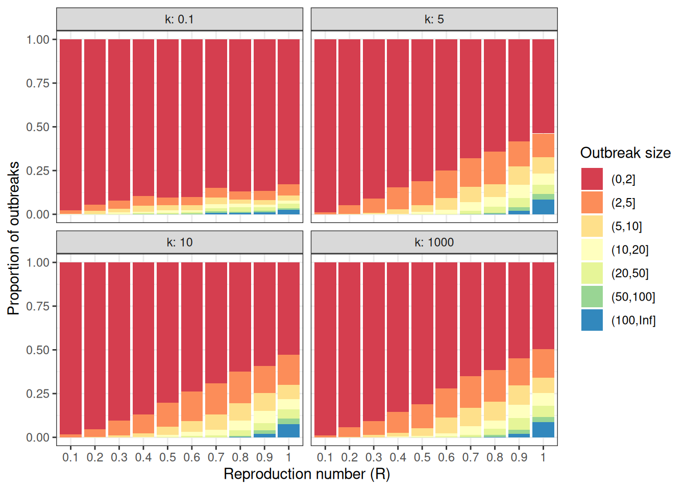
# Change offspring distribution to Negative binomial ----------------------

statistic <- "size"
offspring_dist <- "rnbinom"
R <- seq(0.1, 1.0, 0.1)
k <- c(0.1, 5, 10, 1000)

scenarios <- expand.grid(
  offspring_dist = offspring_dist,
  statistic = statistic,
  R = R,
  k = k,
  stringsAsFactors = FALSE
)

# Simulate outbreak size distribution (Negative binomial) -----------------

outbreak_list <- vector(mode = "list", length = nrow(scenarios))
for (i in seq_len(nrow(scenarios))) {
  offspring_dist_fun <- match.fun(scenarios[i, "offspring_dist"])

  outbreak_list[[i]] <- epichains::simulate_chain_stats(
    n_chains = n_chains,
    statistic = scenarios[i, "statistic"],
    offspring_dist = offspring_dist_fun,
    mu = scenarios[i, "R"],
    size = scenarios[i, "k"],
    stat_threshold = breaks[length(breaks) - 1] + 1
  )
}

# Group outbreak sizes ----------------------------------------------------

intervals <- lapply(outbreak_list, cut, breaks = breaks)

prop <- lapply(intervals, function(interval) {
  table(interval) / sum(table(interval))
})

outbreak_size_list <- lapply(prop, as.data.frame)

for (i in seq_len(nrow(scenarios))) {
  outbreak_size_list[[i]]$R <- scenarios[i, "R"]
  outbreak_size_list[[i]]$k <- scenarios[i, "k"]
  outbreak_size_list[[i]]$offspring_dist <- scenarios[i, "offspring_dist"]
  outbreak_size_list[[i]]$statistic <- scenarios[i, "statistic"]
}

outbreak_size2 <- do.call(rbind, outbreak_size_list)

head(outbreak_size2)
#>   interval  Freq   R   k offspring_dist statistic
#> 1    (0,2] 0.978 0.1 0.1        rnbinom      size
#> 2    (2,5] 0.019 0.1 0.1        rnbinom      size
#> 3   (5,10] 0.002 0.1 0.1        rnbinom      size
#> 4  (10,20] 0.001 0.1 0.1        rnbinom      size
#> 5  (20,50] 0.000 0.1 0.1        rnbinom      size
#> 6 (50,100] 0.000 0.1 0.1        rnbinom      size

# Plot outbreak size distribution (Negative binomial) ---------------------

ggplot2::ggplot(data = outbreak_size2) +
  ggplot2::geom_col(
    mapping = ggplot2::aes(x = as.factor(R), y = Freq, fill = interval)
  ) +
  ggplot2::scale_x_discrete(name = "Reproduction number (R)") +
  ggplot2::scale_y_continuous(name = "Proportion of outbreaks") +
  ggplot2::scale_fill_brewer(
    name = "Outbreak size",
    palette = "Spectral"
  ) +
  ggplot2::facet_wrap(
    facets = c("k"),
    labeller = ggplot2::label_both
  ) +
  ggplot2::theme_bw()

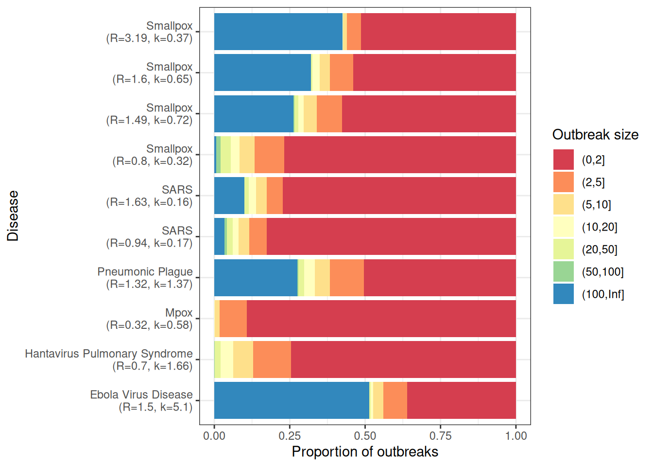
# Simulating outbreak sizes for past outbreaks ----------------------------

offspring_dists <- epiparameter::epiparameter_db(
  epi_name = "offspring distribution"
)

# Check all empirical distributions are the same --------------------------

length(unique(vapply(offspring_dists, family, FUN.VALUE = character(1)))) == 1
#> [1] TRUE

# Simulate empirical outbreak size distributions --------------------------

outbreak_list <- vector(mode = "list", length = length(offspring_dists))

for (i in seq_along(offspring_dists)) {
  offspring_dist_fun <- match.fun(paste0("r", family(offspring_dists[[i]])))

  outbreak_list[[i]] <- epichains::simulate_chain_stats(
    n_chains = n_chains,
    statistic = "size",
    offspring_dist = offspring_dist_fun,
    mu = epiparameter::get_parameters(offspring_dists[[i]])[["mean"]],
    size = epiparameter::get_parameters(offspring_dists[[i]])[["dispersion"]],
    stat_threshold = breaks[length(breaks) - 1] + 1
  )
}

# Group outbreak sizes ----------------------------------------------------

# paste suffix as some diseases have multiple offspring distributions
diseases <- make.unique(
  vapply(offspring_dists, `[[`, FUN.VALUE = character(1), "disease")
)

intervals <- lapply(outbreak_list, cut, breaks = breaks)

prop <- lapply(intervals, function(interval) {
  table(interval) / sum(table(interval))
})

outbreak_size_list <- lapply(prop, as.data.frame)

for (i in seq_along(offspring_dists)) {
  outbreak_size_list[[i]]$R <- epiparameter::get_parameters(offspring_dists[[i]])[["mean"]]
  outbreak_size_list[[i]]$k <- epiparameter::get_parameters(offspring_dists[[i]])[[
    "dispersion"
  ]]
  outbreak_size_list[[i]]$offspring_dist <- family(offspring_dists[[i]])
  outbreak_size_list[[i]]$disease <- diseases[i]
  outbreak_size_list[[i]]$statistic <- "size"
}

outbreak_size3 <- do.call(rbind, outbreak_size_list)

outbreak_size3 <- outbreak_size3 |>
  dplyr::mutate(
    disease = stringr::str_remove(disease, "\\.\\d+$"),
    interval = factor(interval, levels = unique(interval)), # preserve order
    # Create a label combining R and k for each disease
    disease_label = paste0(disease, "\n(R=", R, ", k=", k, ")")
  )

head(outbreak_size3)
#>   interval  Freq    R    k offspring_dist disease statistic
#> 1    (0,2] 0.773 1.63 0.16         nbinom    SARS      size
#> 2    (2,5] 0.054 1.63 0.16         nbinom    SARS      size
#> 3   (5,10] 0.034 1.63 0.16         nbinom    SARS      size
#> 4  (10,20] 0.024 1.63 0.16         nbinom    SARS      size
#> 5  (20,50] 0.015 1.63 0.16         nbinom    SARS      size
#> 6 (50,100] 0.001 1.63 0.16         nbinom    SARS      size
#>            disease_label
#> 1 SARS\n(R=1.63, k=0.16)
#> 2 SARS\n(R=1.63, k=0.16)
#> 3 SARS\n(R=1.63, k=0.16)
#> 4 SARS\n(R=1.63, k=0.16)
#> 5 SARS\n(R=1.63, k=0.16)
#> 6 SARS\n(R=1.63, k=0.16)

# Plot empirical outbreak sizes -------------------------------------------

ggplot2::ggplot(data = outbreak_size3) +
  ggplot2::geom_col(
    mapping = ggplot2::aes(
      x = as.factor(disease_label),
      y = Freq,
      fill = interval
    )
  ) +
  ggplot2::scale_x_discrete(
    name = "Disease"
  ) +
  ggplot2::scale_y_continuous(name = "Proportion of outbreaks") +
  ggplot2::scale_fill_brewer(
    name = "Outbreak size",
    palette = "Spectral"
  ) +
  coord_flip() +
  ggplot2::theme_bw()

Steps in detail

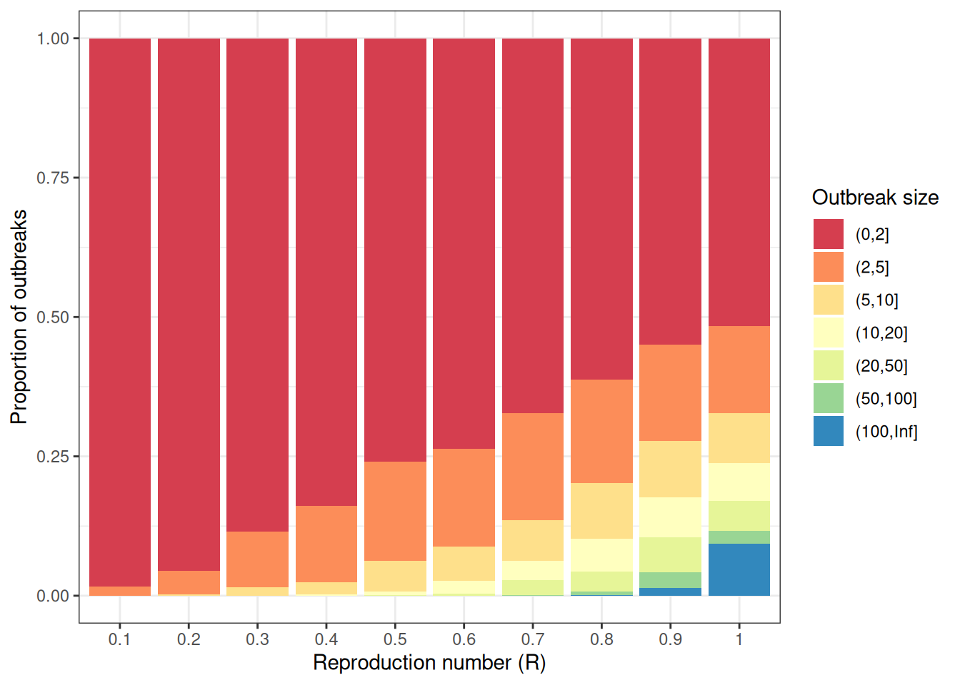
Size is defined as the total number of individuals infected across all generations of infection.

Please note that the code assumes the necessary packages are already installed. If they are not, you can install them using first the install.packages("pak") function and then the pak::pak() function for both packages in CRAN or GitHub before loading them with library().

What do we have?

Steps in code

Steps in detail

Related