How to use epidemics classes with odin-generated models?

Ingredients

This guide shows how to use some of the convenient features of epidemics, especially the classes that describe populations, interventions, and vaccination regimes, with models that are generated by odin.

This guide shows this interoperability by implementing the default model from epidemics in odin.

Steps in code

# Load packages
library(epidemics)
library(socialmixr)
library(odin)
library(data.table)
library(ggplot2)

# Prepare population initial conditions

# get social contacts data
polymod <- socialmixr::polymod
contact_data <- socialmixr::contact_matrix(
  polymod,
  countries = "United Kingdom",
  age.limits = c(0, 20, 40),
  symmetric = TRUE
)

# assume arbitrary populations for each demo group
demography_vector <- contact_data$demography$population

# prepare contact matrix, divide by leading eigenvalue and rowwise by popsize
contact_matrix <- t(contact_data[["matrix"]])
contact_matrix <- (contact_matrix / max(Re(eigen(contact_matrix)$values))) /
  demography_vector

# an intervention to close schools
close_schools <- epidemics::intervention(
  type = "contacts",
  time_begin = 200,
  time_end = 260,
  reduction = base::matrix(c(0.5, 0.01, 0.01))
)

# view the intervention
close_schools
#> 
#>  Intervention name:
#> 
#>  Begins at: 
#> [1] 200
#> 
#>  Ends at: 
#> [1] 260
#> 
#>  Reduction: 
#>              Interv. 1
#> Demo. grp. 1      0.50
#> Demo. grp. 2      0.01
#> Demo. grp. 3      0.01

# initial conditions defined as proportions and converted to absolute values
initial_conditions <- base::matrix(
  c(S = 1 - 1e-6, E = 0, I = 1e-6, R = 0),
  nrow = length(demography_vector),
  ncol = 4L, byrow = TRUE
) * demography_vector

# an intervention to close schools
close_schools <- epidemics::intervention(
  type = "contacts",
  time_begin = 200,
  time_end = 260,
  reduction = base::matrix(c(0.15,0.15,0.15))
)

# view the intervention
close_schools
#> 
#>  Intervention name:
#> 
#>  Begins at: 
#> [1] 200
#> 
#>  Ends at: 
#> [1] 260
#> 
#>  Reduction: 
#>              Interv. 1
#> Demo. grp. 1      0.15
#> Demo. grp. 2      0.15
#> Demo. grp. 3      0.15

# Define an epidemic SEIR model in {odin}
seir <- odin::odin({
  # NOTE: crude time-dependence of transmission rate
  # similar to a `<rate_intervention>`
  beta_reduce[] <- if (t > intervention_interval[1] && t < intervention_interval[2]) (1.0 - reduction[i]) else 1

  # number of age groups taken from contact matrix passed by user
  n <- user()

  # FOI is contacts * infectious * transmission rate
  # returns a matrix, must be converted to a vector/1D array
  lambda_prod[, ] <- C[i, j] * I[j] * beta * beta_reduce[j]* beta_reduce[i]
  #lambda_prod2[, ] <- if (i != j) lambda_prod[i, j] * beta_reduce[i] else lambda_prod[i, j] # if want to keep diagonal the same
  lambda[] <- sum(lambda_prod[i, ])

  ## Derivatives
  deriv(S[]) <- -S[i] * lambda[i]
  deriv(E[]) <- (S[i] * lambda[i]) - (nu * E[i])
  deriv(I[]) <- (nu * E[i]) - (gamma * I[i])
  deriv(R[]) <- gamma * I[i]

  ## Initial conditions: passed by user
  initial(S[]) <- init_S[i]
  initial(E[]) <- init_E[i]
  initial(I[]) <- init_I[i]
  initial(R[]) <- init_R[i]

  ## parameters
  beta <- user()
  nu <- 1 / 3
  gamma <- 1 / 7
  C[, ] <- user() # user defined contact matrix
  init_S[] <- user()
  init_E[] <- user()
  init_I[] <- user()
  init_R[] <- user()
  reduction[] <- user()
  intervention_interval[] <- user()

  # dimensions - all rely on contact matrix
  dim(lambda_prod) <- c(n, n)
  #dim(lambda_prod2) <- c(n, n)
  dim(lambda) <- n
  dim(S) <- n
  dim(E) <- n
  dim(I) <- n
  dim(R) <- n
  dim(init_S) <- n
  dim(init_E) <- n
  dim(init_I) <- n
  dim(init_R) <- n
  dim(reduction) <- n
  dim(beta_reduce) <- n
  dim(C) <- c(n, n)
  dim(intervention_interval) <- 2
})

# Initialise model and run over time 0 - 600
mod <- seir$new(
  beta = 1.5 / 7,
  reduction = close_schools$reduction[,],
  intervention_interval = c(close_schools$time_begin, close_schools$time_end),
  C = contact_matrix, n = nrow(contact_matrix),
  init_S = initial_conditions[, 1],
  init_E = initial_conditions[, 2],
  init_I = initial_conditions[, 3],
  init_R = initial_conditions[, 4]
)
t <- seq(0, 600)
y <- mod$run(t)

# convert to data.table and plot infectious in each age class
y <- as.data.table(y)
y <- melt(y, id.vars = c("t"))

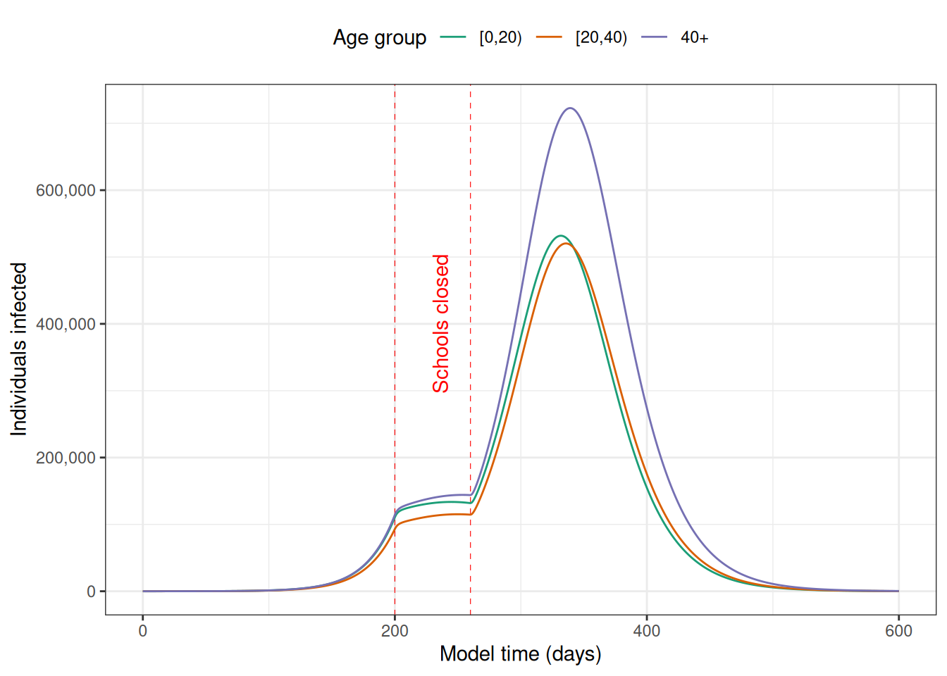
ggplot(y[variable %like% "I"]) +
  geom_vline(
    xintercept = c(close_schools[["time_begin"]], close_schools[["time_end"]]),
    colour = "red",
    linetype = "dashed",
    linewidth = 0.2
  ) +
  annotate(
    geom = "text",
    label = "Schools closed",
    colour = "red",
    x = 230, y = 400e3,
    angle = 90,
    vjust = "outward"
  ) +
  geom_line(
    aes(t, value, col = variable) 
  ) +
  scale_colour_brewer(
    palette = "Dark2",
    labels = rownames(contact_matrix),
    name = "Age group"
  ) +
  scale_y_continuous(
    labels = scales::comma,
    name = "Individuals infected"
  ) +
  labs(
    x = "Model time (days)"
  ) +
  theme_bw() +
  theme(
    legend.position = "top"
  )