Modelling disease control interventions

epichains does not provide any direct functionality for studying reductions in transmission (e.g. from public health interventions). However, the flexible simulation functionality that it includes can be used to consider some specific changes to the parameters that can be interpreted as the result of changes in social behaviour or control measures. Here we investigate the effect on outbreak sizes, but the same approaches could be used for investigating chain lengths (using the statistic argument to simulate_chain_stats()) or the time progression of outbreaks (using the simulate_chains() function).

Some of the ideas presented here can be achieved using closed-form solutions of the probability of an epidemic growing out of proportion or going extinct, and the impact of heterogeneities in individual-level transmission. For examples of this, see the vignette on epidemic risk in the superspreading package, which is part of the Epiverse-TRACE Initiative.

## main package
library("epichains")
## for plotting
library("ggplot2")
## for truncating the offspring distribution later
library("truncdist")

As a base case we consider the spread of an infection with a negative binomial offspring distribution with mean 1.2 and overdispersion parameter 0.5. We simulate 200 chains tracking up to 99 infections:

sims <- simulate_chain_stats(
  n_chains = 200, offspring_dist = rnbinom, stat_threshold = 99, mu = 1.2,
  size = 0.5, statistic = "size"
)

We then plot the resulting distribution of chain sizes

sims[is.infinite(sims)] <- 100 # Replace infections > 99 with 100 for plotting.
ggplot(data.frame(x = sims), aes(x = x)) +
  geom_histogram(breaks = seq(0, 100, by = 5), closed = "left") +
  scale_x_continuous(breaks = c(0, 25, 50, 75, 100),
                     labels = c(0, 25, 50, 75, ">99")) +
  theme_bw()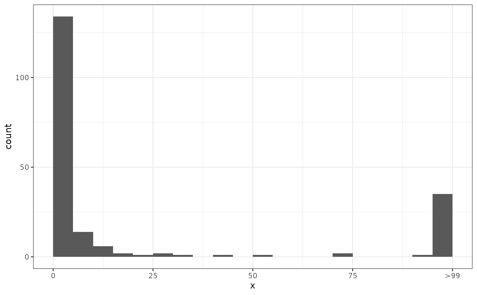

Reducing the strength of transmission

Following (Lloyd-Smith et al. 2005) we consider two ways in which disease control interventions can reduce the reproduction number: population-wide and individual-specific control.

Population-wide control

By population-level control we mean an intervention that reduces the mean number of offspring (i.e. the reproduction number) by a fixed proportion. For example, to reduce R by 25% at the population level we scale the mu parameter from 1.2 to 0.9:

sims <- simulate_chain_stats(
  n_chains = 200, offspring_dist = rnbinom, stat_threshold = 99, mu = 0.9,
  size = 0.5, statistic = "size"
)
sims[is.infinite(sims)] <- 100 # Replace infections > 99 with 100 for plotting.
ggplot(data.frame(x = sims), aes(x = x)) +
  geom_histogram(breaks = seq(0, 100, by = 5), closed = "left") +
  scale_x_continuous(breaks = c(0, 25, 50, 75, 100),
                     labels = c(0, 25, 50, 75, ">99")) +
  theme_bw()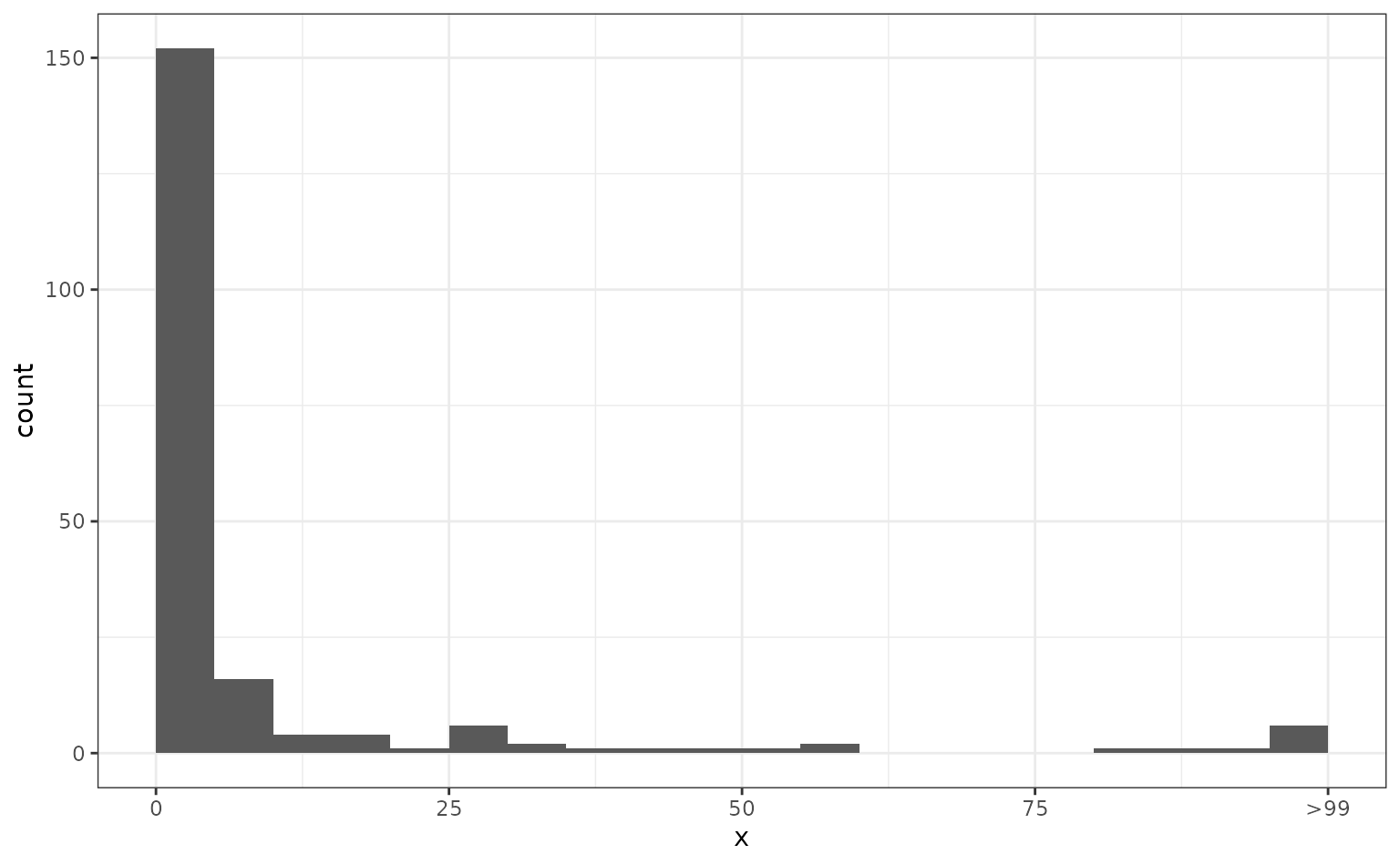

Individual-level control.

In simulating population-level control we now apply the same reduction as before (25%) but instead of assuming that the mean is reduced we apply this such that 25% of individuals do not transmit further at all, whereas the remaining 75% generate offspring as in the uncontrolled case.

To do this, we can no longer use the standard negative binomial distribution that comes with R. Instead, we define a random generator from a modified negative binomial distribution that includes our individual-level control as a control argument indicating the level of individual-level control (0: no control; 1: full control):

rnbinom_ind <- function(n, ..., control = 0) {
  ## initialise number of offspring to 0
  offspring <- rep(0L, n)
  ## for each individual, decide whether they transmit further
  transmits <- rbinom(n = n, prob = 1 - control, size = 1)
  ## check if anyone transmits further
  if (any(transmits == 1L)) {
    ## for those that transmit, sample from negative binomial with given
    ## parameters
    offspring[which(transmits == 1L)] <- rnbinom(n = n, ...)
  }
  return(offspring)
}

Having defined this, we can generate simulations as before:

sims <- simulate_chain_stats(
  n_chains = 200, offspring_dist = rnbinom_ind, stat_threshold = 99, mu = 1.2,
  size = 0.5, control = 0.25, statistic = "size"
)
sims[is.infinite(sims)] <- 100 # Replace infections > 99 with 100 for plotting.
ggplot(data.frame(x = sims), aes(x = x)) +
  geom_histogram(breaks = seq(0, 100, by = 5), closed = "left") +
  scale_x_continuous(breaks = c(0, 25, 50, 75, 100),
                     labels = c(0, 25, 50, 75, ">99")) +
  theme_bw()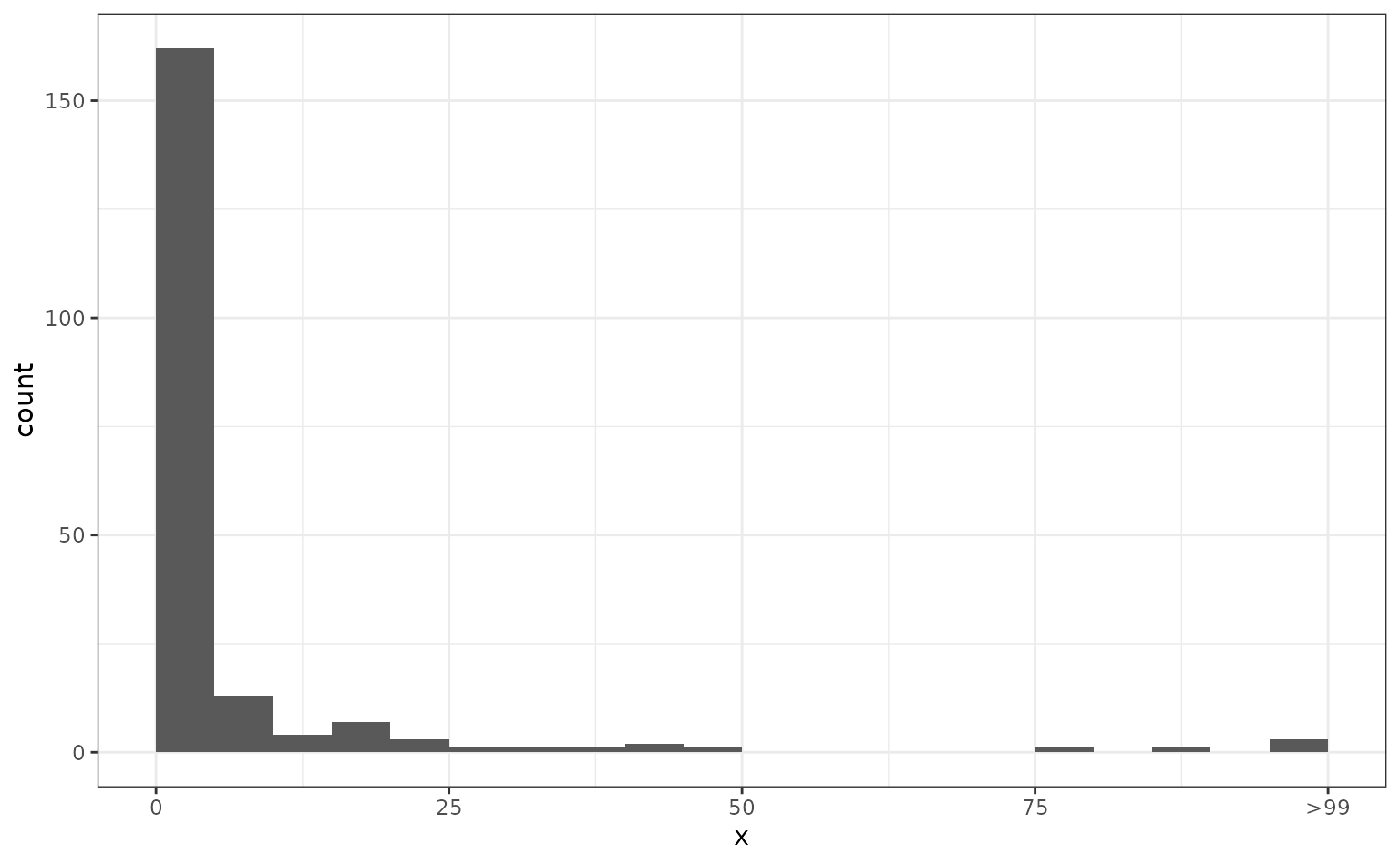

Preventing superspreading events

Another way of controlling a disease would be to prevent individuals from spreading to a large number of others, for example by preventing mass gatherings or, more generally, settings where superspreading events can occur.

We can model this by truncating the offspring distribution at a certain size. This can be done, for example, using the truncdist R package. We use this to define a truncated negative binomial offspring distribution:

rnbinom_truncated <- function(n, ..., max = Inf) {
  return(rtrunc(n = n, spec = "nbinom", b = max, ...))
}

We use this to simulate chains in a situation where the maximum of secondary cases that each infected person can generate is 10. This can be likened to a disease control strategy where gatherings are limited to 10 people.

sims <- simulate_chain_stats(
  n_chains = 200, offspring_dist = rnbinom_truncated, stat_threshold = 99,
  mu = 1.2, size = 0.5, max =  10, statistic = "size"
)
sims[is.infinite(sims)] <- 100 # Replace infections > 99 with 100 for plotting.
ggplot(data.frame(x = sims), aes(x = x)) +
  geom_histogram(breaks = seq(0, 100, by = 5), closed = "left") +
  scale_x_continuous(breaks = c(0, 25, 50, 75, 100),
                     labels = c(0, 25, 50, 75, ">99")) +
  theme_bw()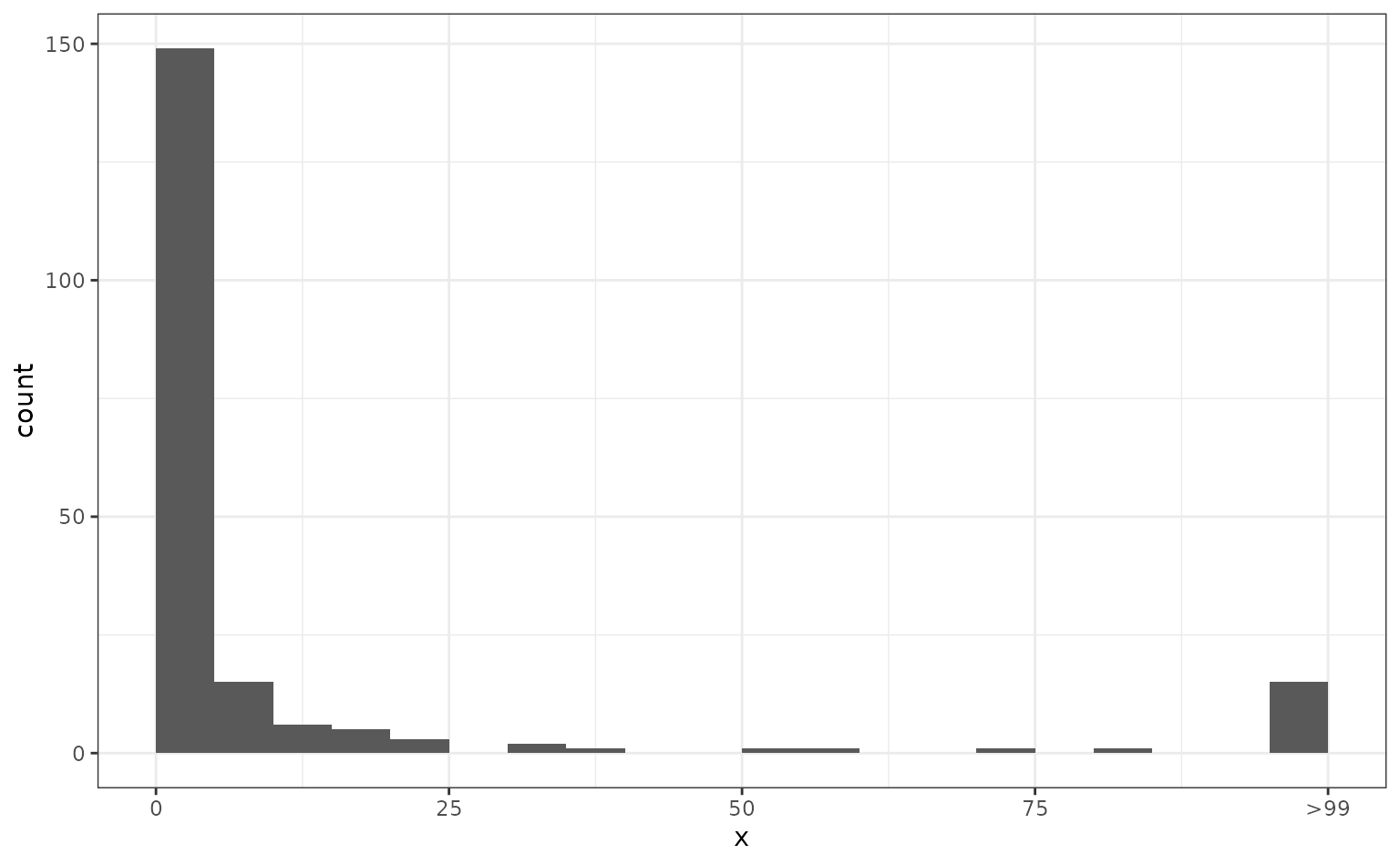

Truncating the generation interval

Lastly, we consider a situation where the generation interval is shortened. We do not model this explicitly but instead consider the effect on the offspring distribution.

For example, if our generation interval is from a gamma distribution with shape = 25 and rate = 5 (corresponding to a mean of 5 and standard deviation of 1), and we stop all transmission that would normally occur more than 6 days after infection, we can calculate the proportion of transmissions that are prevented as

control <- 1 - pgamma(6, shape = 25, rate = 5)
signif(control, 2)
#> [1] 0.16

In other words, this would prevent 16% of infections in this example. The value of control can be used in the examples above to study the effect on outbreak sizes.

References