Estimation of force of infection from serological surveys using serofoi
Last updated on 2026-04-28 | Edit this page
Estimated time: 55 minutes
Overview
Questions
- How to retrospectively estimate the Force of Infection of a pathogen from age-disaggregated population-based serological prevalence surveys by implementing Bayesian models using serofoi?
Objectives
At the end of this workshop you will be able to:
Explore and analyze a typical serological survey.
Learn how to estimate the Infection Strength in a specific use case.
Visualize and interpret the results.
1. Introduction
serofoi is an R package for retrospectively estimating the Force of Infection of a pathogen from age-disaggregated population-based serological prevalence surveys by implementing Bayesian models. For this purpose, serofoi uses the Rstan package, which provides an interface to the statistical programming language Stan, through which Monte-Carlo methods based on Markov chains are implemented.
As a particular case, we will study an outbreak of Chikungunya, a viral disease discovered in Tanzania in 1952 that is characterized by severe fevers, joint pain, headache, rashes, among other symptoms. Since 2013, cases of this disease began to be reported in the Americas and since then the disease has been endemic in several Latin American countries. During this tutorial, we will analyze a serological survey conducted between October and December 2015 in Bahia, Brazil, which was conducted shortly after an epidemic of this disease, in order to characterize the endemic or epidemic patterns in the area.
2. Objectives
Explore and analyze a typical serological survey.
Learn how to estimate the Infection Strength in a specific use case.
Visualize and interpret the results.
3. Basic concepts to be developed
The following concepts will be developed in this practice:
Serological surveys (sero)
Infection strength (foi)
Serocatalytic models
Bayesian Statistics
Visualization and interpretation of FoI model results
The Force of Infection (FoI), also known as the risk rate or infection pressure, represents the rate at which susceptible individuals become infected given exposure to a pathogen. In other words, FoI quantifies the risk of a susceptible individual becoming infected over a period of time.
As we will see below, this concept is key in modeling infectious diseases. To illustrate the concept, let us consider a population exposed to a pathogen and call \(P(t)\) the proportion of individuals that have been infected at time \(t\). Assuming no sero-reversion, the quantity \(1 - P(t)\) represents the number of individuals susceptible to the disease, such that the rate of infection is given by:
\[ \tag{1} \frac{dP(t)}{d t} = \lambda(t) (1- P(t)), \]
where \(lambda(t)\) represents the rate at which susceptible individuals become infected per unit time (days, months, years, …), i.e. FoI. The differential equation (1) resembles that of a chemical reaction where \(P(t)\) represents the proportion of substrate that has not come into contact with a catalytic reagent, so these types of models are known as serocatalytic models (Muench, 1959).
Despite the simplicity of the model represented by equation (1), compared to compartmental models (for example), the difficulty in knowing an initial condition for seropositivity at some point in the past makes its practical use impossible. To circumvent this limitation, it is common to apply the model for age cohorts rather than for the total population. To do this, let us label each age cohort according to its year of birth \(tau\), and assume that individuals are seronegative at birth:
\[ \frac{dP^\tau (t)}{dt} = \lambda(t) (1 - P^\tau(t)). \]
With initial conditions given by \(P^\tau(\tau) = 0\). This equation can be solved analytically, yielding the result (Hens et al, 2010):
\[ P^{\tau} (t) = 1 - \exp\left(-\int_{\tau}^{t} \lambda (t') dt' \right). \]
Assuming that FoI remains constant throughout each year, the discrete version of this equation is:
\[ \tag{2} P^\tau(t) = 1 - \exp\left(-\sum_{i = \tau}^{t} \lambda_i \right), \]
As an example, consider the FoI represented in the following figure:
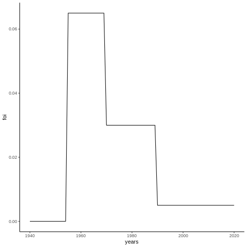
From this FoI, it is possible to calculate the seroprevalence for different cohorts by means of equation (2):
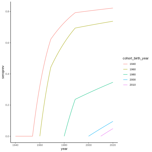
When we know the data from a serological survey, the information we have access to is a snapshot of the seroprevalence at the time \(t_{sur}\) as a function of the age of the individuals at that time, which coincides with equation (2) since individuals age at the same rate as time passes; that is:
\[ \tag{3} P^{t_{sur}}(a^\tau) = 1 - \exp\left(-\sum_{i = \tau}^{t_{sur}} \lambda_i \right). \]
In the case of the example, this gives us the following graph:
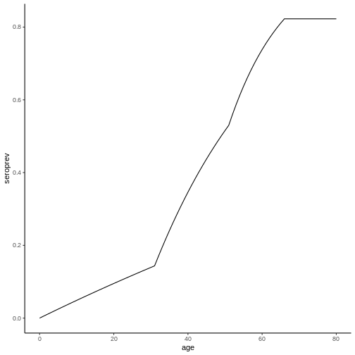
Note that the seroprevalence values for each age in this graph correspond to the seroprevalence values at the time of the survey (2020) in the previous graph.
The mission that serofoi fulfills is to estimate the historical force of infection \("tambda(t)\) from this snapshot of the serologic profile of the population at the time of the survey. for which serologic surveys that meet the following inclusion criteria are required:
- Population-based (non-hospital).
- Cross-sectional study (single time).
- Indicate the diagnostic test used.
- Identifying the patient’s age at the time of the survey.
In cases where FoI can be considered constant, equation (3) gives the result:
\[ \tag{4} P_{sur}(a^\tau(t_{sur})) = 1 - \exp (-\lambda a^\tau), \]
where it was taken into account that, at the time of pathogen introduction (\(t = 0\)), the proportion of infected individuals was \(P(0) = 0\) (initial condition). Note that the summation term in equation (3) results in the age of each cohort when considering constant force of infection.

Figure 1. Prevalence curves as a function of age for different values of constant FoI.
In this example we have chosen, for simplicity, that the FoI was constant; however, this is not necessarily the case. Identifying whether the FoI follows a constant or time-varying trend can be of vital importance in identifying and characterizing the spread of a disease. This is where the R serofoi package plays an important role, as it allows to retrospectively estimate the FoI of a pathogen, thus recovering its temporal evolution, by means of pre-established Bayesian models.
Current models in the serofoi package assume the following biological assumptions:
- No sero-reversion (no loss of immunity).
- FoI is not age-dependent.
- Low or no levels of migration in the populations.
- Small differences between susceptible and infected mortality rates. infected.
3.2. Bayesian models
Unlike the frequentist approach, where the probability is associated with the relative frequency of occurrence of events, Bayesian statistics is based on the use of the conditional probability of events with respect to the knowledge (or state of information) that we may have about the data or about the parameters we want to estimate.
In general, when we propose a model what we seek is to reduce the uncertainty about some parameter, so that we approach its value as optimally as our previous knowledge of the phenomenon and the measurements (data) allow us to do.
Bayesian inference is supported by Bayes’ theorem, which states that: given a data set \(\vec{y} = (y_1, ..., y_N)\), which represents a single event, and the random variable \(\theta\), which represents a parameter of interest to us (in our case, the FoI \(\lambda\)), the joint probability distribution of the associated random variables is given by:
\[ \tag{4} p(\vec{y}, \theta) = p(\vec{y} | \theta) p(\theta) = p(\theta | \vec{y}) p(\vec{y}), \]
from which we derive the aposteriori distribution of \(\theta\), i.e. an updated version of the FoI probability distribution conditional on our data:
\[\tag{5} p(\theta, \vec{y}) = \frac{p(\vec{y} | \theta) p(\theta)}{p(\vec{y})}, \]
The distribution \(p(\vec{y} | \theta)\), which corresponds to the information internal to the data conditional on the value of the parameter \(\theta\), is usually determined by the nature of the experiment: it is not the same to choose balls inside a box by replacing them than by leaving them outside the box (e.g.). In the particular case of FoI, we have data such as the total number of surveys by age and the number of positive cases, so it is reasonable to assign a binomial distribution to the probability, as we will see below.
3.3.1. Constant FoI model
In our particular case, the parameter that we want to estimate is the FoI (\(\lambda\)). The apriori probability distribution of \(\lambda\) represents our informed assumptions or the prior knowledge we have about the behavior of the FoI. In this context, the state of minimal information about \(\lambda\) is represented by a uniform distribution:
\[\tag{6} \lambda \sim U(0, 2), \]
which means that we start from the premise that all values of the force of infection between \(0\) and \(2\) are equally probable. On the other hand, from the theory of sero-catalytic models we know that seroprevalence in a given year is described by a cumulative process with age (Hens et al, 2010):
\[\tag{7} P(a, t) = 1 - \exp\left( -\sum_{i=t-a+1}^{t} \lambda_i \right), \]
where \(\lambda_i\) corresponds to the FoI at time \(t\). Since in this case the FoI is constant, eq. (7) reduces to:
\[\tag{8} P(a, t) = 1 - \exp\left( -\lambda a \right), \]
If \(n(a, t_{sur})\) is the number of age-positive samples obtained in a serological study conducted in the year \(t_{sur}\), then we can estimate the distribution of age-positive cases conditional on the value of \(t_{sur}\) as a binomial distribution:
\[\tag{9} p(a, t) \sim Binom(n(a, t), P(a, t)) \\ \lambda \sim U(0, 2) \]
3.3.2. Time-dependent FOI Model
Currently, serofoi allows the implementation of two time-dependent models: one for slow variation of FoI (time) and one for fast variation (time-log) of FoI.
Each of them is based on different prior distributions for \(lambda\), which are shown in Table 1.
| Model Type | Model Type | Logarithmic Scale | Probability of positive case at age \(a\) |
|---|---|---|---|
"constant" |
FALSE |
\(\sim binom(n(a,t), P(a,t))\) | \(\lambda\sim uniform(0,2)\) |
"time" |
FALSE |
\(\sim binom(n(a,t), P(a,t))\) | \(\lambda\sim normal(\lambda(t-1),\sigma)\ \lambda(t=1)\sim normal(0,1)\) |
"time" |
TRUE |
\(\sim binom(n(a,t), P(a,t))\) | \(\lambda\sim normal(log(\lambda(t-1)),\sigma)\ \lambda(t=1)\sim normal(-6,4)\) |
Table 1. A priori distributions of the different models supported by serofoi. \(sigma\) represents the standard deviation.
As can be seen, the prior distributions of \(\lambda\) in both cases are given by
Gaussian distributions with standard deviation \(\sigma\) and centered on \(\lambda\) (slow-variation model -
"time") and \(\log(\lambda)\) (fast-variation model -
"time" with is_log_foi = TRUE). Thus, the FoI
at time \(t\) is distributed according
to a normal distribution around the value it had at the immediately
preceding time. The logarithm in the \(log(\lambda)\) model allows to identify
drastic changes in the time trend of FoI.
Workshop content
4.1 serofoi installation
Prior to the installation of serofoi, create an R project in the folder of your choice on your local machine; this in order to organize the workspace where the codes you develop during the session will be stored.
Before installing serofoi, it is necessary to install and configure C++ Toolchain (instructions for windows/ mac/ linux).
Windows users will need a working installation of Rtools
in order to build the package from source. Rtools is not an
R package, but a software you need to download and install. We suggest
you to follow:
-
Verify
Rtoolsinstallation. You can do so by using Windows search across your system. Optionally, you can use devtools running:
R
if(!require("devtools")) install.packages("devtools")
devtools::find_rtools()
If the result is FALSE, then you should do step 2.
Install
Rtools. Download theRtoolsinstaller from https://cran.r-project.org/bin/windows/Rtools/. Install with default selections.Verify
Rtoolsinstallation. Again, we can use devtools:
R
if(!require("devtools")) install.packages("devtools")
devtools::find_rtools()
After you have configured C++ Toolchain, run the following lines of code to install the package:
R
if(!require("pak")) install.packages("pak")
pak::pak("serofoi")
If you get an error, your can try:
R
install.packages("serofoi")
Optionally, it is possible to modify the R configuration so that the models to be implemented run in parallel, taking advantage of the processor cores of your computer. This has the effect of reducing the computation time of the implementations in Stan. To activate this option run:
R
options(mc.cores=parallel::detectCores())
Finally, load the package by running
R
library(serofoi)
4.2 Use case: Chikungunya
In this section we will analyze a serological survey conducted
between October and December 2015 in Bahia, Brazil, which was carried
out shortly after an epidemic of this disease in the area. Our objective
is to characterize the spread of the disease by implementing the
different models and determine which of these best describes the
situation. First, let us load and prepare the data that we will use in
this analysis. The database chik2015 contains the data
corresponding to this serological survey:
R
data(chik2015)
chik2015
OUTPUT
  survey_year n_sample n_seropositive age_min age_max
1        2015      144             63      40      59
2        2015      148             69      60      79
3        2015       45             17       1      19
4        2015      109             55      20      39
To run the constant FoI model and visualize the results of the model, run the following lines of code:
R
chik_constant <- fit_seromodel(serosurvey = chik2015,
                               model_type = "constant",
                               iter = 1000)

chik_constant_plot <- plot_seromodel(seromodel = chik_constant,
                                     serosurvey = chik2015,
                                     size_text = 12)
Now, run the time-dependent models with iter =1500. Then
visualize the three plots together using the plot_grid()
function of the cowplot package:
R
install.packages("cowplot")

cowplot::plot_grid(chik_constant_plot,
                   chik_normal_plot,
                   chik_normal_log_plot,
                   ncol = 3)
NOTE: . Because the number of trajectories is relatively high, in order to ensure convergence of the models, the computation time of the time-dependent models may take several minutes.
Hint: You should get the following graph: * Hint: You should get the following graph: * Hint: You should get the following graph

The predictive power of a Bayesian model can be characterized by the elpd(Expected Log Predictive Density). The model that best fits the epidemiological survey is the one that has higher values of elpd and lower values of standard error (se).
Comparison of the models
The predictive power of a Bayesian model can be characterized by means of the elpd (Expected Log Predictive Density), which corresponds to the expected value of the log-likelihood (log-likelihood) of a single new data \(y'\) with respect to its real distribution (which we want to approximate with the model):
\[ \text{elpd} = \mathbb{E}_{\text{real}}[\log(p(y'|\vec{y}))] = \int p^{\text{real}}(y') \log(p(y'|\vec{y})) \, dy' \]
where \(\vec{y}\) corresponds to the data.
There are several methods for estimating the elpd that allow to approximate the predictive accuracy of a Bayesian model. The Watanabe-Akaike information criterion (WAIC) is one of them:
\[ \text{WAIC} = -2 \hat{lpd} + 2 p_{\text{waic}} \]
where \(p_{{text{waic}}\) is the effective number of parameters and \({hat{lpd}}\) corresponds to the logarithm of the average likelihood with respect to the posterior distribution for a data \(y_i \in \vec{y}\):
\[ \hat{lpd} = \log(\mathbb{E}_{\text{post}}[p(y_i|\theta)]) \]
The purpose of subtracting the effective number of parameters from the model is to account for the possibility of overfitting the model. The WAIC allows us to characterize the predictive capacity of the model: the lower its value, the better.
Similarly, we can compute the looic (leave-one-out information criterion), also known as loo-cv (leave-one-out cross-validation), which consists of using a single data point to test the predictive power of the model using the rest of the sample as the training sample. This process is repeated with each data point in the sample and their respective log posterior densities are summed (Lambert 2018), ie:
\[ \text{looic} = \sum_{y_i} \log(p(y_i | \vec{y}_{i})) \]
where \(\vec{y}_{i}\) represents the data sample extracting \(y_i\).
5. Reflection
Discussion
According to the criteria explained above, please answer:
Which of the three models best fits this serological survey?
How do you interpret these results?
Challenge: simulated case
The challenge is carried out with 4 teams (each of 4-5 people), which will be supported by a coordinator and 4 monitors.
Each team must generate a diagnosis of the situation in the different regions, as well as compare the evolution of the disease in order to evaluate the control strategies in each region.
Source: Reto
Challenge
Challenge: simulated case
In the past 3 years, cases of encephalitis of unknown origin have been identified in humans in rural border areas of two neighboring Latin American countries. Some of these cases of encephalitis have required hospitalization and even deaths have been reported. Locals also point out that a similar epidemic of cases in which people*“lost consciousness after a high fever”* had occurred in the same area a few decades earlier.
In 2023, a seroprevalence survey was conducted for the 4 viruses most suspected to be circulating in the border area where encephalitis cases occur. These 4 viruses are biologically distinct from each other, i.e. they do not cross-react in serological tests. For each of these viruses, the seroprevalence survey collected a probabilistic and representative sample of the population of residents of the area with a total of 1306 individuals sampled between 1 and 60 years of age. The results of the serological tests for each virus are presented as the total number of people sampled for each age group and the number of people positive for IgG antibodies against one of the 4 viruses in that age group.
The challenge is for you and your group to identify which of the 4 viruses is most likely to be involved in this viral encephalitis emergency using the serofoi library.
Data exploration and visualization of seroprevalence (30 min).
The data from the 4 surveys come in separate . RDS files that you can find in these links:
- https://epiverse-trace.github.io/epimodelac/data/serosurvey_01.RDS
- https://epiverse-trace.github.io/epimodelac/data/serosurvey_02.RDS
- https://epiverse-trace.github.io/epimodelac/data/serosurvey_03.RDS
- https://epiverse-trace.github.io/epimodelac/data/serosurvey_04.RDS
Read the data using the readRDS() function. At this
stage of the challenge you are expected to:
Explore the structure of the data and discuss the general characteristics of an age-disaggregated cross-sectional serological survey.
Prepare the data for the visualization process by means of functions from the dplyr package.
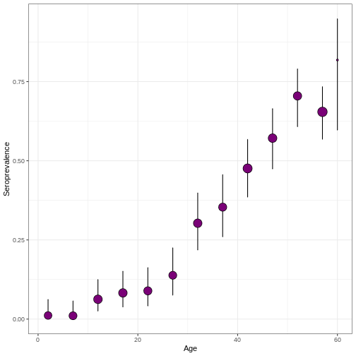
Visualize the seroprevalence of each survey by means of the
plot_seroprev() function and qualitatively analyze its
trend in each case.
Estimation of the historical force of infection (30 min).
Implement the models you consider relevant to each serological survey and compare the results obtained using Bayesian comparison metrics. At this stage it is expected that:
Implement the Bayesian models available in serofoi by means of the
fit_seromodel()function. How does using more or fewer
iterations affect your results?
- Comparison of the fits obtained by means of the
plot_seromodel()function. Which model fits best in each case?
Results analysis (30 min)
Based on the results obtained above, which virus do you think was involved in the recent encephalitis epidemic?
To adapt one of the four databases to the format required for {serofoi}, you can use the following code:
R
library(tidyverse)

virus_serosurvey <- readr::read_rds(
  "https://epiverse-trace.github.io/epimodelac/data/serosurvey_01.RDS"
) %>%
  dplyr::mutate(
    age_group = vaccineff::get_age_group(
      data_set = .,
      col_age = "age_max",
      max_val = 60,
      step = 5
    )
  ) %>%
  dplyr::group_by(age_group, survey_year = tsur) %>%
  dplyr::summarise(
    n_sample = sum(total),
    n_seropositive = sum(counts),
    age_min = min(age_min),
    age_max = max(age_max)
  ) %>%
  dplyr::ungroup() %>%
  dplyr::select(-age_group)
Now, how would you implement the Bayesian models available in serofoi
via the fit_seromodel() function?
Sample solution for a database:
R
virus_serosurvey %>%
  serofoi::plot_serosurvey()
R
virus_serosurvey %>%
  serofoi::fit_seromodel(model_type = "time", iter = 1000) %>%
  serofoi::plot_seromodel(serosurvey = virus_serosurvey)
OUTPUT
SAMPLING FOR MODEL 'time_no_seroreversion' NOW (CHAIN 1).
Chain 1:
Chain 1: Gradient evaluation took 9.5e-05 seconds
Chain 1: 1000 transitions using 10 leapfrog steps per transition would take 0.95 seconds.
Chain 1: Adjust your expectations accordingly!
Chain 1:
Chain 1:
Chain 1: Iteration:   1 / 1000 [  0%]  (Warmup)
Chain 1: Iteration: 100 / 1000 [ 10%]  (Warmup)
Chain 1: Iteration: 200 / 1000 [ 20%]  (Warmup)
Chain 1: Iteration: 300 / 1000 [ 30%]  (Warmup)
Chain 1: Iteration: 400 / 1000 [ 40%]  (Warmup)
Chain 1: Iteration: 500 / 1000 [ 50%]  (Warmup)
Chain 1: Iteration: 501 / 1000 [ 50%]  (Sampling)
Chain 1: Iteration: 600 / 1000 [ 60%]  (Sampling)
Chain 1: Iteration: 700 / 1000 [ 70%]  (Sampling)
Chain 1: Iteration: 800 / 1000 [ 80%]  (Sampling)
Chain 1: Iteration: 900 / 1000 [ 90%]  (Sampling)
Chain 1: Iteration: 1000 / 1000 [100%]  (Sampling)
Chain 1:
Chain 1:  Elapsed Time: 3.712 seconds (Warm-up)
Chain 1:                2.183 seconds (Sampling)
Chain 1:                5.895 seconds (Total)
Chain 1:

SAMPLING FOR MODEL 'time_no_seroreversion' NOW (CHAIN 2).
Chain 2:
Chain 2: Gradient evaluation took 8.6e-05 seconds
Chain 2: 1000 transitions using 10 leapfrog steps per transition would take 0.86 seconds.
Chain 2: Adjust your expectations accordingly!
Chain 2:
Chain 2:
Chain 2: Iteration:   1 / 1000 [  0%]  (Warmup)
Chain 2: Iteration: 100 / 1000 [ 10%]  (Warmup)
Chain 2: Iteration: 200 / 1000 [ 20%]  (Warmup)
Chain 2: Iteration: 300 / 1000 [ 30%]  (Warmup)
Chain 2: Iteration: 400 / 1000 [ 40%]  (Warmup)
Chain 2: Iteration: 500 / 1000 [ 50%]  (Warmup)
Chain 2: Iteration: 501 / 1000 [ 50%]  (Sampling)
Chain 2: Iteration: 600 / 1000 [ 60%]  (Sampling)
Chain 2: Iteration: 700 / 1000 [ 70%]  (Sampling)
Chain 2: Iteration: 800 / 1000 [ 80%]  (Sampling)
Chain 2: Iteration: 900 / 1000 [ 90%]  (Sampling)
Chain 2: Iteration: 1000 / 1000 [100%]  (Sampling)
Chain 2:
Chain 2:  Elapsed Time: 3.31 seconds (Warm-up)
Chain 2:                2.943 seconds (Sampling)
Chain 2:                6.253 seconds (Total)
Chain 2:

SAMPLING FOR MODEL 'time_no_seroreversion' NOW (CHAIN 3).
Chain 3:
Chain 3: Gradient evaluation took 8.7e-05 seconds
Chain 3: 1000 transitions using 10 leapfrog steps per transition would take 0.87 seconds.
Chain 3: Adjust your expectations accordingly!
Chain 3:
Chain 3:
Chain 3: Iteration:   1 / 1000 [  0%]  (Warmup)
Chain 3: Iteration: 100 / 1000 [ 10%]  (Warmup)
Chain 3: Iteration: 200 / 1000 [ 20%]  (Warmup)
Chain 3: Iteration: 300 / 1000 [ 30%]  (Warmup)
Chain 3: Iteration: 400 / 1000 [ 40%]  (Warmup)
Chain 3: Iteration: 500 / 1000 [ 50%]  (Warmup)
Chain 3: Iteration: 501 / 1000 [ 50%]  (Sampling)
Chain 3: Iteration: 600 / 1000 [ 60%]  (Sampling)
Chain 3: Iteration: 700 / 1000 [ 70%]  (Sampling)
Chain 3: Iteration: 800 / 1000 [ 80%]  (Sampling)
Chain 3: Iteration: 900 / 1000 [ 90%]  (Sampling)
Chain 3: Iteration: 1000 / 1000 [100%]  (Sampling)
Chain 3:
Chain 3:  Elapsed Time: 3.348 seconds (Warm-up)
Chain 3:                3.137 seconds (Sampling)
Chain 3:                6.485 seconds (Total)
Chain 3:

SAMPLING FOR MODEL 'time_no_seroreversion' NOW (CHAIN 4).
Chain 4:
Chain 4: Gradient evaluation took 8.7e-05 seconds
Chain 4: 1000 transitions using 10 leapfrog steps per transition would take 0.87 seconds.
Chain 4: Adjust your expectations accordingly!
Chain 4:
Chain 4:
Chain 4: Iteration:   1 / 1000 [  0%]  (Warmup)
Chain 4: Iteration: 100 / 1000 [ 10%]  (Warmup)
Chain 4: Iteration: 200 / 1000 [ 20%]  (Warmup)
Chain 4: Iteration: 300 / 1000 [ 30%]  (Warmup)
Chain 4: Iteration: 400 / 1000 [ 40%]  (Warmup)
Chain 4: Iteration: 500 / 1000 [ 50%]  (Warmup)
Chain 4: Iteration: 501 / 1000 [ 50%]  (Sampling)
Chain 4: Iteration: 600 / 1000 [ 60%]  (Sampling)
Chain 4: Iteration: 700 / 1000 [ 70%]  (Sampling)
Chain 4: Iteration: 800 / 1000 [ 80%]  (Sampling)
Chain 4: Iteration: 900 / 1000 [ 90%]  (Sampling)
Chain 4: Iteration: 1000 / 1000 [100%]  (Sampling)
Chain 4:
Chain 4:  Elapsed Time: 3.13 seconds (Warm-up)
Chain 4:                2.555 seconds (Sampling)
Chain 4:                5.685 seconds (Total)
Chain 4:
WARNING
Warning: There were 3 divergent transitions after warmup. See
https://mc-stan.org/misc/warnings.html#divergent-transitions-after-warmup
to find out why this is a problem and how to eliminate them.
WARNING
Warning: There were 1 chains where the estimated Bayesian Fraction of Missing Information was low. See
https://mc-stan.org/misc/warnings.html#bfmi-low
WARNING
Warning: Examine the pairs() plot to diagnose sampling problemsWARNING
Warning: Bulk Effective Samples Size (ESS) is too low, indicating posterior means and medians may be unreliable.
Running the chains for more iterations may help. See
https://mc-stan.org/misc/warnings.html#bulk-ess
WARNING
Warning: Tail Effective Samples Size (ESS) is too low, indicating posterior variances and tail quantiles may be unreliable.
Running the chains for more iterations may help. See
https://mc-stan.org/misc/warnings.html#tail-ess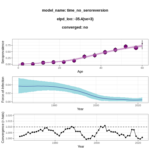
Key Points
Check if you have acquired these competencies at the end of this lesson:
Explore and analyze a typical serological survey.
Learn how to estimate the Infection Strength in a specific use case.
Visualize and interpret the results.
About this document
This document has been designed for the International Course: Outbreak Analysis and Modeling in Public Health, Bogotá 2023. TRACE-LAC/Javeriana.
Contributions
- Nicolás Torres Domínguez
- Zulma M. Cucunuba
Contributions are welcome via pull requests.
References
Muench, H. (1959). Catalytic models in epidemiology. Harvard University Press.
Hens, N., Aerts, M., Faes, C., Shkedy, Z., Lejeune, O., Van Damme, P., Beutels, P. (2010). Seventy-five years of estimating the force of infection from current status data. Epidemiology & Infection, 138(6), 802-812.
Cucunubá, Z. M., Nouvellet, P., Conteh, L., Vera, M. J., Angulo, V. M., Dib, J. C., … Basáñez, M. G. (2017). Modelling historical changes in the force-of-infection of Chagas disease to inform control and elimination programmes: application in Colombia. BMJ Global Health, 2(3). doi:10.1136/bmjgh-2017-000345.