Instructor Notes
This is a placeholder file. Please add content here.
Estimation of force of infection from serological surveys using serofoi
Instructor Note
Comparison of the models
The predictive power of a Bayesian model can be characterized by means of the elpd (Expected Log Predictive Density), which corresponds to the expected value of the log-likelihood (log-likelihood) of a single new data \(y'\) with respect to its real distribution (which we want to approximate with the model):
\[ \text{elpd} = \mathbb{E}_{\text{real}}[\log(p(y'|\vec{y}))] = \int p^{\text{real}}(y') \log(p(y'|\vec{y})) \, dy' \]
where \(\vec{y}\) corresponds to the data.
There are several methods for estimating the elpd that allow to approximate the predictive accuracy of a Bayesian model. The Watanabe-Akaike information criterion (WAIC) is one of them:
\[ \text{WAIC} = -2 \hat{lpd} + 2 p_{\text{waic}} \]
where \(p_{{text{waic}}\) is the effective number of parameters and \({hat{lpd}}\) corresponds to the logarithm of the average likelihood with respect to the posterior distribution for a data \(y_i \in \vec{y}\):
\[ \hat{lpd} = \log(\mathbb{E}_{\text{post}}[p(y_i|\theta)]) \]
The purpose of subtracting the effective number of parameters from the model is to account for the possibility of overfitting the model. The WAIC allows us to characterize the predictive capacity of the model: the lower its value, the better.
Similarly, we can compute the looic (leave-one-out information criterion), also known as loo-cv (leave-one-out cross-validation), which consists of using a single data point to test the predictive power of the model using the rest of the sample as the training sample. This process is repeated with each data point in the sample and their respective log posterior densities are summed (Lambert 2018), ie:
\[ \text{looic} = \sum_{y_i} \log(p(y_i | \vec{y}_{i})) \]
where \(\vec{y}_{i}\) represents the data sample extracting \(y_i\).
Instructor Note
Challenge: simulated case
The challenge is carried out with 4 teams (each of 4-5 people), which will be supported by a coordinator and 4 monitors.
Each team must generate a diagnosis of the situation in the different regions, as well as compare the evolution of the disease in order to evaluate the control strategies in each region.
Source: Reto
Instructor Note
Sample solution for a database:
R
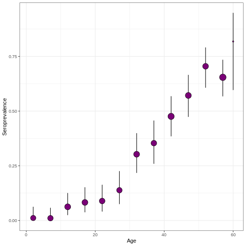
virus_serosurvey %>%
  serofoi::plot_serosurvey()
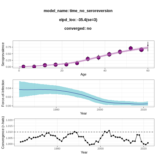
R
virus_serosurvey %>%
  serofoi::fit_seromodel(model_type = "time", iter = 1000) %>%
  serofoi::plot_seromodel(serosurvey = virus_serosurvey)
OUTPUT
SAMPLING FOR MODEL 'time_no_seroreversion' NOW (CHAIN 1).
Chain 1:
Chain 1: Gradient evaluation took 9.5e-05 seconds
Chain 1: 1000 transitions using 10 leapfrog steps per transition would take 0.95 seconds.
Chain 1: Adjust your expectations accordingly!
Chain 1:
Chain 1:
Chain 1: Iteration:   1 / 1000 [  0%]  (Warmup)
Chain 1: Iteration: 100 / 1000 [ 10%]  (Warmup)
Chain 1: Iteration: 200 / 1000 [ 20%]  (Warmup)
Chain 1: Iteration: 300 / 1000 [ 30%]  (Warmup)
Chain 1: Iteration: 400 / 1000 [ 40%]  (Warmup)
Chain 1: Iteration: 500 / 1000 [ 50%]  (Warmup)
Chain 1: Iteration: 501 / 1000 [ 50%]  (Sampling)
Chain 1: Iteration: 600 / 1000 [ 60%]  (Sampling)
Chain 1: Iteration: 700 / 1000 [ 70%]  (Sampling)
Chain 1: Iteration: 800 / 1000 [ 80%]  (Sampling)
Chain 1: Iteration: 900 / 1000 [ 90%]  (Sampling)
Chain 1: Iteration: 1000 / 1000 [100%]  (Sampling)
Chain 1:
Chain 1:  Elapsed Time: 3.712 seconds (Warm-up)
Chain 1:                2.183 seconds (Sampling)
Chain 1:                5.895 seconds (Total)
Chain 1:

SAMPLING FOR MODEL 'time_no_seroreversion' NOW (CHAIN 2).
Chain 2:
Chain 2: Gradient evaluation took 8.6e-05 seconds
Chain 2: 1000 transitions using 10 leapfrog steps per transition would take 0.86 seconds.
Chain 2: Adjust your expectations accordingly!
Chain 2:
Chain 2:
Chain 2: Iteration:   1 / 1000 [  0%]  (Warmup)
Chain 2: Iteration: 100 / 1000 [ 10%]  (Warmup)
Chain 2: Iteration: 200 / 1000 [ 20%]  (Warmup)
Chain 2: Iteration: 300 / 1000 [ 30%]  (Warmup)
Chain 2: Iteration: 400 / 1000 [ 40%]  (Warmup)
Chain 2: Iteration: 500 / 1000 [ 50%]  (Warmup)
Chain 2: Iteration: 501 / 1000 [ 50%]  (Sampling)
Chain 2: Iteration: 600 / 1000 [ 60%]  (Sampling)
Chain 2: Iteration: 700 / 1000 [ 70%]  (Sampling)
Chain 2: Iteration: 800 / 1000 [ 80%]  (Sampling)
Chain 2: Iteration: 900 / 1000 [ 90%]  (Sampling)
Chain 2: Iteration: 1000 / 1000 [100%]  (Sampling)
Chain 2:
Chain 2:  Elapsed Time: 3.31 seconds (Warm-up)
Chain 2:                2.943 seconds (Sampling)
Chain 2:                6.253 seconds (Total)
Chain 2:

SAMPLING FOR MODEL 'time_no_seroreversion' NOW (CHAIN 3).
Chain 3:
Chain 3: Gradient evaluation took 8.7e-05 seconds
Chain 3: 1000 transitions using 10 leapfrog steps per transition would take 0.87 seconds.
Chain 3: Adjust your expectations accordingly!
Chain 3:
Chain 3:
Chain 3: Iteration:   1 / 1000 [  0%]  (Warmup)
Chain 3: Iteration: 100 / 1000 [ 10%]  (Warmup)
Chain 3: Iteration: 200 / 1000 [ 20%]  (Warmup)
Chain 3: Iteration: 300 / 1000 [ 30%]  (Warmup)
Chain 3: Iteration: 400 / 1000 [ 40%]  (Warmup)
Chain 3: Iteration: 500 / 1000 [ 50%]  (Warmup)
Chain 3: Iteration: 501 / 1000 [ 50%]  (Sampling)
Chain 3: Iteration: 600 / 1000 [ 60%]  (Sampling)
Chain 3: Iteration: 700 / 1000 [ 70%]  (Sampling)
Chain 3: Iteration: 800 / 1000 [ 80%]  (Sampling)
Chain 3: Iteration: 900 / 1000 [ 90%]  (Sampling)
Chain 3: Iteration: 1000 / 1000 [100%]  (Sampling)
Chain 3:
Chain 3:  Elapsed Time: 3.348 seconds (Warm-up)
Chain 3:                3.137 seconds (Sampling)
Chain 3:                6.485 seconds (Total)
Chain 3:

SAMPLING FOR MODEL 'time_no_seroreversion' NOW (CHAIN 4).
Chain 4:
Chain 4: Gradient evaluation took 8.7e-05 seconds
Chain 4: 1000 transitions using 10 leapfrog steps per transition would take 0.87 seconds.
Chain 4: Adjust your expectations accordingly!
Chain 4:
Chain 4:
Chain 4: Iteration:   1 / 1000 [  0%]  (Warmup)
Chain 4: Iteration: 100 / 1000 [ 10%]  (Warmup)
Chain 4: Iteration: 200 / 1000 [ 20%]  (Warmup)
Chain 4: Iteration: 300 / 1000 [ 30%]  (Warmup)
Chain 4: Iteration: 400 / 1000 [ 40%]  (Warmup)
Chain 4: Iteration: 500 / 1000 [ 50%]  (Warmup)
Chain 4: Iteration: 501 / 1000 [ 50%]  (Sampling)
Chain 4: Iteration: 600 / 1000 [ 60%]  (Sampling)
Chain 4: Iteration: 700 / 1000 [ 70%]  (Sampling)
Chain 4: Iteration: 800 / 1000 [ 80%]  (Sampling)
Chain 4: Iteration: 900 / 1000 [ 90%]  (Sampling)
Chain 4: Iteration: 1000 / 1000 [100%]  (Sampling)
Chain 4:
Chain 4:  Elapsed Time: 3.13 seconds (Warm-up)
Chain 4:                2.555 seconds (Sampling)
Chain 4:                5.685 seconds (Total)
Chain 4:
WARNING
Warning: There were 3 divergent transitions after warmup. See
https://mc-stan.org/misc/warnings.html#divergent-transitions-after-warmup
to find out why this is a problem and how to eliminate them.
WARNING
Warning: There were 1 chains where the estimated Bayesian Fraction of Missing Information was low. See
https://mc-stan.org/misc/warnings.html#bfmi-low
WARNING
Warning: Examine the pairs() plot to diagnose sampling problemsWARNING
Warning: Bulk Effective Samples Size (ESS) is too low, indicating posterior means and medians may be unreliable.
Running the chains for more iterations may help. See
https://mc-stan.org/misc/warnings.html#bulk-ess
WARNING
Warning: Tail Effective Samples Size (ESS) is too low, indicating posterior variances and tail quantiles may be unreliable.
Running the chains for more iterations may help. See
https://mc-stan.org/misc/warnings.html#tail-ess