Ready reckoner for R_eff

library(finalsize)
library(dplyr)
#> 
#> Attaching package: 'dplyr'
#> The following objects are masked from 'package:stats':
#> 
#>     filter, lag
#> The following objects are masked from 'package:base':
#> 
#>     intersect, setdiff, setequal, union
library(tidyr)
library(ggplot2)

The finalsize package provides a quick way to calculate the effective reproduction number using the r_eff() function. This vignette shows how to use the contact_scaling argument to calculate the effective reproduction number for different scenarios.

Setup

We access social contacts data for the U.K. for six age groups: three school-age groups of 0 – 4, 5 – 11, 12 – 17, and three adult groups of 18 – 39, 40 – 65, and 65+.

Age groups are chosen to model the effect of school closures and resulting reduction in social contacts for school-age groups on $R_\text{eff}$.

We assume all age groups are completely susceptible to infection.

polymod <- socialmixr::polymod
contact_data <- socialmixr::contact_matrix(
  polymod,
  countries = "United Kingdom",
  age.limits = c(0, 5, 12, 17, 40, 65),
  symmetric = TRUE
)
#> Removing participants that have contacts without age information. To change this behaviour, set the 'missing.contact.age' option
#> Warning in pop_age(survey.pop, part.age.group.present, ...): Not all age groups represented in population data (5-year age band).
#>   Linearly estimating age group sizes from the 5-year bands.

# get the contact matrix and demography data
contact_matrix <- t(contact_data$matrix)
demography_vector <- contact_data$demography$population

# scale the contact matrix so the largest eigenvalue is 1.0
# this is to ensure that the overall epidemic dynamics correctly reflect
# the assumed value of R0
contact_matrix <- contact_matrix / max(Re(eigen(contact_matrix)$values))

# divide each row of the contact matrix by the corresponding demography
# this reflects the assumption that each individual in group {j} make contacts
# at random with individuals in group {i}
contact_matrix <- contact_matrix / demography_vector

n_demo_grps <- length(demography_vector)

# all individuals are equally and highly susceptible
n_susc_groups <- 1L
susc_guess <- 1.0

susc_uniform <- matrix(
  data = susc_guess,
  nrow = n_demo_grps,
  ncol = n_susc_groups
)

p_susc_uniform <- matrix(
  data = 1.0,
  nrow = n_demo_grps,
  ncol = n_susc_groups
)

Scenarios of contact reduction

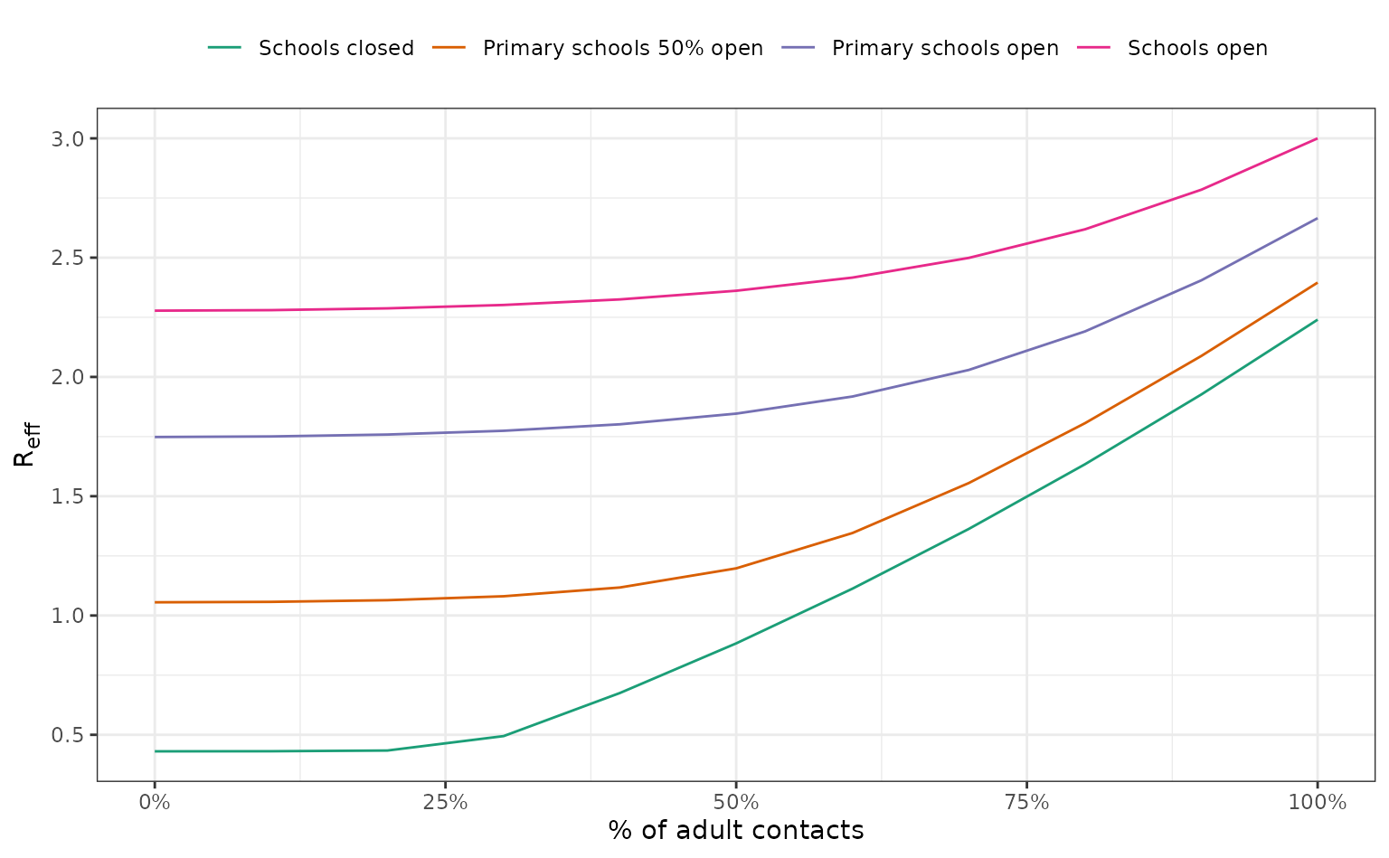
We model four scenarios of school closures, and multiple levels of scaling of adult social contacts.

Note that all values and assumptions are solely illustrative.

# create an age-specific scaling vector for re-use
scaling_factor <- rep(1, n_demo_grps)

# adult age groups
i_adult <- c(4, 5, 6)

n_school_age <- 3L

We assume that:

1. Full school closures reduce all school-age groups’ contacts by 80%;

2. 0-5 year olds’ contacts are not affected in any other scenario;

3. When 50% of 5-11 year olds are at school, contacts are reduced by 40%;

4. 12-17 year olds have an 80% reduction in contacts except when all schools are open;

5. Adults’ social contacts are not affected by school closures.

# create scenarios of school closures
scenarios <- factor(
  c("schools_closed", "ps_half_open", "ps_open", "schools_open"),
  levels = c("schools_closed", "ps_half_open", "ps_open", "schools_open")
)

scenario_names <- c(
  "Schools closed", "Primary schools 50% open",
  "Primary schools open", "Schools open"
)

school_scaling <- list(
  schools_closed = rep(0.2, n_school_age), # full closure cuts contacts by 80%
  ps_half_open = c(1.0, 0.6, 0.2), # 50% 5-11 yr olds cuts contacts by 40%
  ps_open = c(1.0, 1.0, 0.2),
  schools_open = rep(1.0, n_school_age)
)

# make a tibble and cross-join with scaling values
scenarios <- tibble(
  scenarios,
  school_scaling
)

scaling_values <- seq(0.0, 1.0, 0.1) # adult scaling from 0% - 100%

scenarios <- crossing(
  scenarios, scaling_values
)

# combine adult and school-age contact scaling values for 4 * 11 scenarios
scenarios <- mutate(
  scenarios,
  contact_scaling = Map(
    school_scaling, scaling_values,
    f = function(x, y) {
      scaling_factor <- c(x, rep(y, 3)) # all adult contacts scaled the same
    }
  )
)

# calculate R_eff assuming R0 = 3.0
r0 <- 3.0

scenarios <- mutate(
  scenarios,
  r_eff = vapply(
    contact_scaling,
    function(x) {
      r_eff(
        r0,
        contact_matrix, demography_vector, susc_uniform,
        p_susc_uniform,
        contact_scaling = x
      )
    }, numeric(1)
  )
)

We plot the $R_\text{eff}$ values.

ggplot(scenarios) +
  geom_line(
    aes(scaling_values, r_eff, col = scenarios)
  ) +
  scale_color_brewer(
    palette = "Dark2",
    labels = scenario_names
  ) +
  scale_x_continuous(
    labels = scales::percent
  ) +
  scale_y_continuous(
    breaks = seq(0.5, 3, 0.5)
  ) +
  theme_bw() +
  labs(
    x = "% of adult contacts",
    y = "R<sub>eff</sub>",
    colour = NULL
  ) +
  theme(
    axis.title.y.left = ggtext::element_markdown(),
    legend.position = "top"
  )