# Pandemic scenarios with uncertainty -----------------------------------------
# Load packages
library(epidemics)
library(EpiEstim) # for Rt estimation
library(tidyverse)
library(withr)
# Generate an R estimate with EpiEstim ----------------------------------------
# get 2009 influenza data from school in Pennsylvania
data(Flu2009)
flu_early_data <- dplyr::filter(Flu2009$incidence, dates < "2009-05-10")
# define a PDF for the distribution of serial intervals
serial_pdf <- dgamma(seq(0, 25), shape = 2.622, scale = 0.957)
# ensure probabilities add up to 1 by normalising them by the sum
serial_pdf <- serial_pdf / sum(serial_pdf)
# Use EpiEstim to estimate R with uncertainty
# Uses Gamma distribution by default
output_R <- EpiEstim::estimate_R(
incid = flu_early_data,
method = "non_parametric_si",
config = make_config(list(si_distr = serial_pdf))
)
# Plot output to visualise
# plot(output_R, "R")
# get mean mean and sd over time
r_estimate_mean <- mean(output_R$R$`Mean(R)`)
r_estimate_sd <- mean(output_R$R$`Std(R)`)
# Generate 100 R samples
r_samples <- withr::with_seed(
seed = 1,
code = rnorm(
n = 100,
mean = r_estimate_mean,
sd = r_estimate_sd
)
)
# Set up the transmission model -------------------------------------------
# load contact and population data from socialmixr::polymod
polymod <- socialmixr::polymod
contact_data <- socialmixr::contact_matrix(
polymod,
countries = "United Kingdom",
age.limits = c(0, 20, 40), # use three age groups
symmetric = TRUE
)
# prepare contact matrix and demography vector for use in model
# transpose so R0 calculated correctly inside model
contact_matrix <- t(contact_data$matrix)
demography_vector <- contact_data$demography$population
names(demography_vector) <- rownames(contact_matrix)
# initial conditions
initial_i <- 1e-6
initial_conditions <- c(
S = 1 - initial_i, E = 0, I = initial_i, R = 0, V = 0
)
# define same ICs for all age groups
initial_conditions <- rbind(
initial_conditions,
initial_conditions,
initial_conditions
)
# assign rownames for clarity
rownames(initial_conditions) <- rownames(contact_matrix)
# define UK population object
uk_population <- epidemics::population(
name = "UK",
contact_matrix = contact_matrix,
demography_vector = demography_vector,
initial_conditions = initial_conditions
)
# Simulate scenario with uncertainty --------------------------------------
# define epidemic parameters
infectious_period <- 7
beta <- r_samples / infectious_period
# pass the vector of transmissibilities to the basic {epidemics} model
output <- epidemics::model_default(
population = uk_population,
transmission_rate = beta,
recovery_rate = 1 / infectious_period,
time_end = 600
)
# select the parameter set and data columns with dplyr::select()
# add the R value for visualisation
# calculate new infections, and use tidyr to unnest the data column
data <- dplyr::select(output, param_set, transmission_rate, data) %>%
mutate(
r_value = r_samples,
new_infections = purrr::map(data, new_infections)
) %>%
dplyr::select(-data) %>%
tidyr::unnest(new_infections)
# Plot outputs ------------------------------------------------------------
# # plot the data
# data %>%
# dplyr::filter() %>%
# ggplot() +
# geom_line(
# aes(time, new_infections, col = r_value, group = param_set),
# alpha = 0.3
# ) +
# # use qualitative scale to emphasize differences
# scale_colour_fermenter(
# palette = "Dark2",
# name = "R",
# breaks = c(0, 1, 1.5, 2.0, 3.0),
# limits = c(0, 3)
# ) +
# scale_y_continuous(
# name = "New infections",
# labels = scales::label_comma(scale = 1e-3, suffix = "K")
# ) +
# labs(
# x = "Time (days since start of epidemic)"
# ) +
# facet_grid(
# cols = vars(demography_group)
# ) +
# theme_bw() +
# theme(
# legend.position = "top",
# legend.key.height = unit(2, "mm")
# )
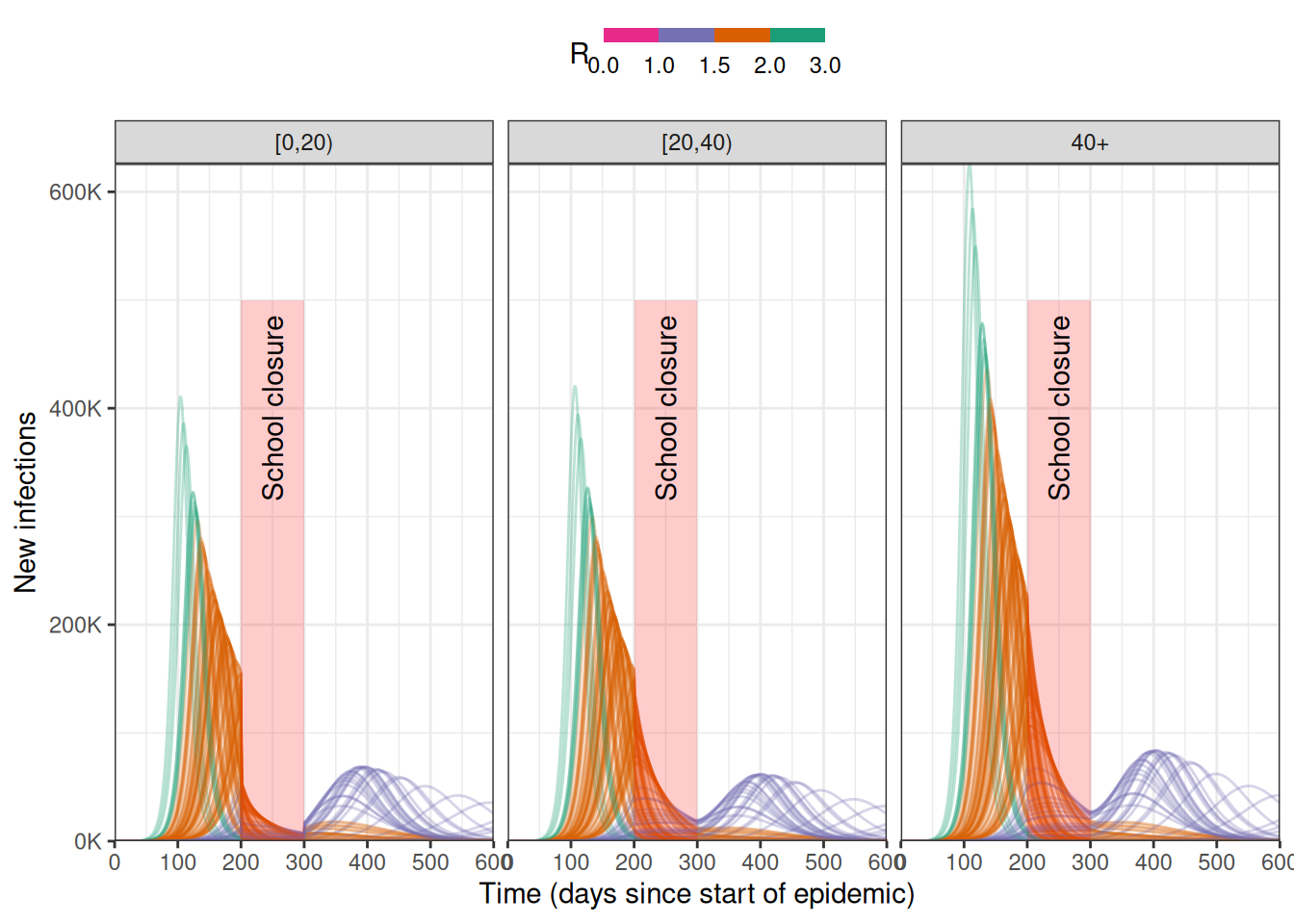
# Add an intervention -----------------------------------------------------
# prepare a school-closure intervention with a differential effect on age groups
close_schools <- epidemics::intervention(
name = "School closure",
type = "contacts",
time_begin = 200,
time_end = 300,
reduction = matrix(c(0.5, 0.001, 0.001))
)
# run model with intervention
output <- epidemics::model_default(
population = uk_population,
transmission_rate = beta,
recovery_rate = 1 / infectious_period,
intervention = list(contacts = close_schools),
time_end = 600
)
# reformat data for plotting
data <- dplyr::select(output, param_set, transmission_rate, data) %>%
dplyr::mutate(
r_value = r_samples,
new_infections = map(data, new_infections)
) %>%
dplyr::select(-data) %>%
tidyr::unnest(new_infections)
# plot the data
data %>%
dplyr::filter() %>%
ggplot() +
geom_line(
aes(time, new_infections, col = r_value, group = param_set),
alpha = 0.3
) +
# use qualitative scale to emphasize differences
scale_colour_fermenter(
palette = "Dark2",
name = "R",
breaks = c(0, 1, 1.5, 2.0, 3.0),
limits = c(0, 3)
) +
scale_y_continuous(
name = "New infections",
labels = scales::label_comma(scale = 1e-3, suffix = "K")
) +
labs(
x = "Time (days since start of epidemic)"
) +
facet_grid(
cols = vars(demography_group)
) +
theme_bw() +
theme(
legend.position = "top",
legend.key.height = unit(2, "mm")
) +
annotate(
geom = "rect",
xmin = close_schools$time_begin,
xmax = close_schools$time_end,
ymin = 0, ymax = 500e3,
fill = alpha("red", alpha = 0.2),
lty = "dashed"
) +
annotate(
geom = "text",
x = mean(c(close_schools$time_begin, close_schools$time_end)),
y = 400e3,
angle = 90,
label = "School closure"
) +
expand_limits(
y = c(0, 500e3)
) +
coord_cartesian(
expand = FALSE
)