Modelling overlapping and sequential interventions targeting social contacts • epidemics

New to epidemics, or to modelling non-pharmaceutical interventions? It may help to read the “Get started” and “Modelling a non-pharmaceutical intervention targeting social contacts” vignettes first!

Code

library(epidemics)
library(ggplot2)

Prepare population and initial conditions

We prepare population and contact data from the U.K., with epidemiological compartments matching the default epidemic model (SEIR-V).

We assume that one in every million people has been infected and is infectious, translating to about 67 total infections for a U.K. population of 67 million.

The code for these steps is similar to that in the “Getting started vignette” and is hidden here, although it can be expanded for reference.

Code

# load contact and population data from socialmixr::polymod
polymod <- socialmixr::polymod
contact_data <- socialmixr::contact_matrix(
  polymod,
  countries = "United Kingdom",
  age.limits = c(0, 20, 65),
  symmetric = TRUE
)

# prepare contact matrix
contact_matrix <- t(contact_data$matrix)

# prepare the demography vector
demography_vector <- contact_data$demography$population
names(demography_vector) <- rownames(contact_matrix)

Code

# initial conditions
initial_i <- 1e-4
initial_conditions <- c(
  S = 1 - initial_i, E = 0, I = initial_i, R = 0, V = 0
)

# build for all age groups
initial_conditions <- rbind(
  initial_conditions,
  initial_conditions,
  initial_conditions
)

# assign rownames for clarity
rownames(initial_conditions) <- rownames(contact_matrix)

Code

uk_population <- population(
  name = "UK",
  contact_matrix = contact_matrix,
  demography_vector = demography_vector,
  initial_conditions = initial_conditions
)

Examine the baseline

We first examine the baseline scenario — no interventions are implemented to slow the spread of the epidemic — and visualise the outcomes in terms of daily new infections.

We simulate an epidemic using model_default(), calling the default model outlined in the “Get started vignette”.

Code

# no intervention baseline scenario
data_baseline <- model_default(
  population = uk_population,
  time_end = 400, increment = 1.0
)

# get new infections
data_baseline_infections <- new_infections(data_baseline, by_group = TRUE)

We show one instance of the plotting code using the ggplot2 package here, with further instances hidden to keep the vignette short.

Code

# visualise the spread of the epidemic in terms of new infections
# plot figure of epidemic curve
plot_baseline <- ggplot() +
  geom_line(
    data = data_baseline_infections,
    aes(time, new_infections, colour = demography_group),
    linetype = "dashed"
  ) +
  scale_y_sqrt(
    labels = scales::comma,
    breaks = c(10^seq(3, 5), 5e4)
  ) +
  scale_colour_brewer(
    palette = "Dark2",
    name = "Age group"
  ) +
  coord_cartesian(
    expand = FALSE
  ) +
  theme_bw() +
  theme(
    legend.position = "top"
  ) +
  labs(
    x = "Simulation time (days)",
    linetype = "Compartment",
    y = "Individuals"
  )

plot_baseline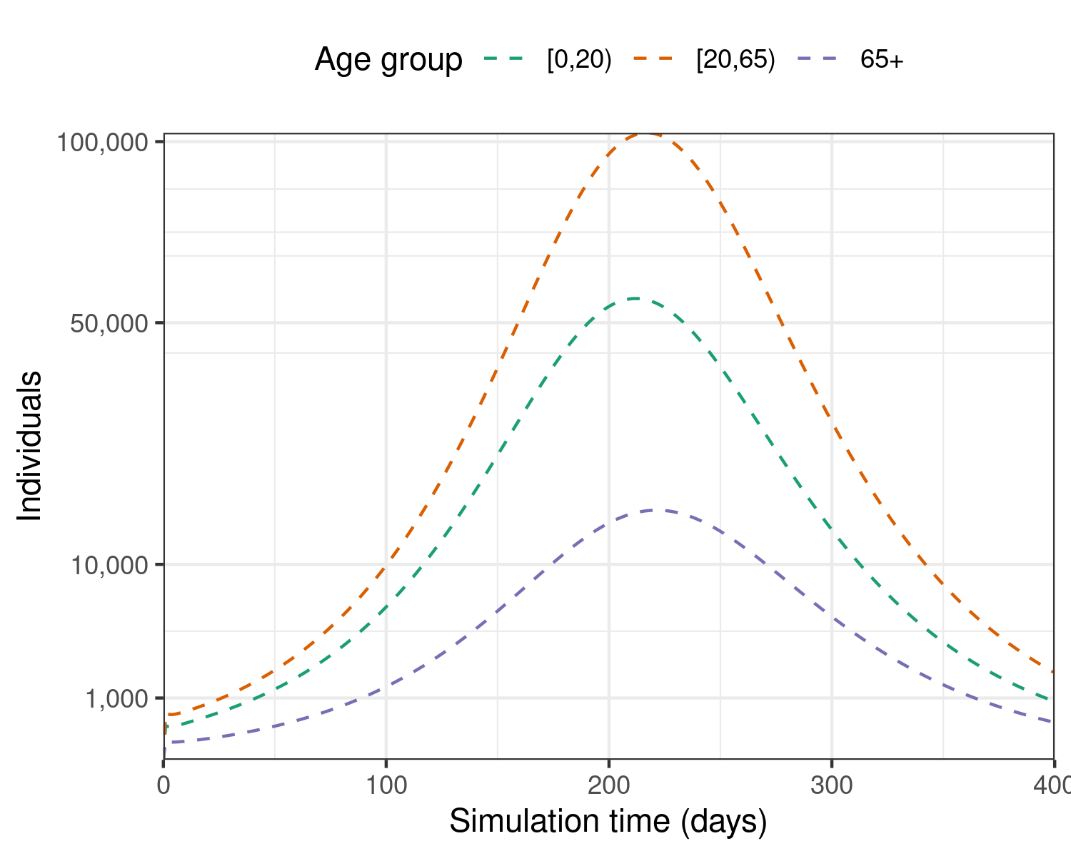

A model of an infectious disease epidemic, assuming a directly transmitted infection such as influenza, with an $R_0$ of 1.3, an infectious period of 5 days, and a pre-infectious period of 1.5 days.

Figure 1: A model of an infectious disease epidemic, assuming a directly transmitted infection such as influenza, with an $R_0$ of 1.3, an infectious period of 5 days, and a pre-infectious period of 1.5 days.

In the baseline scenario, the epidemic would continue for approximately 400 days, or more than one year, with a peak in new infections between the 150th and 180th day for the different age groups.

In this scenario, the epidemic is expected to have a final size of around 23 million individuals infected overall.

In the following sections we shall iteratively model the effects of applying non-pharmaceutical interventions that reduce contacts to examine whether the epidemic’s final size could be reduced, and whether the peak of infections can be spread out over time.

Modelling overlapping interventions

We shall prepare multiple interventions that could plausibly implemented over the course of an epidemic.

School closures

In the first example, we shall model school closures, which are primarily aimed at reducing infections among younger individuals who could then transmit them to their families.

We first prepare an intervention that simulates the effect of closing schools to reduce the contacts of younger people. We assume that this reduces the contacts of the age group 0 – 19 by 30%, and the contacts of all other age groups by only 1% (as most adults meet individuals their own age).

This intervention is assumed to last 6 months or approximately 180 days, beginning from the 100th day of the outbreak — this is similar to the duration of initial school closures during the Covid-19 pandemic in 2020 in the U.K.

Code

# prepare an intervention that models school closures for ~3 months (100 days)
close_schools <- intervention(
  name = "School closure",
  type = "contacts",
  time_begin = 60,
  time_end = 60 + 180,
  reduction = matrix(c(0.3, 0.01, 0.01))
)

# examine the intervention object
close_schools
#> 
#>  Intervention name: 
#>  Begins at: 
#> [1] 60
#> 
#>  Ends at: 
#> [1] 240
#> 
#>  Reduction: 
#>              Interv. 1
#> Demo. grp. 1      0.30
#> Demo. grp. 2      0.01
#> Demo. grp. 3      0.01

We simulate the epidemic for 600 days as we expect the intervention to spread disease incidence out over a longer period.

Code

# no intervention baseline scenario
data_schools_closed <- model_default(
  population = uk_population,
  intervention = list(contacts = close_schools),
  time_end = 600, increment = 1.0
)

# get new infections
data_noschool_infections <- new_infections(data_schools_closed, by_group = TRUE)

Code

# visualise the spread of the epidemic in terms of new infections when
# schools are closed
plot_noschool <-
  ggplot() +
  geom_vline(
    xintercept = c(
      close_schools$time_begin,
      close_schools$time_end
    ),
    linetype = "dotted"
  ) +
  annotate(
    geom = "text",
    x = mean(c(close_schools$time_begin, close_schools$time_end)),
    y = 1000,
    label = "Schools closed"
  ) +
  geom_line(
    data = data_baseline_infections,
    aes(time, new_infections, colour = demography_group),
    linetype = "dashed"
  ) +
  geom_line(
    data = data_noschool_infections,
    aes(time, new_infections, colour = demography_group),
    linetype = "solid"
  ) +
  scale_y_sqrt(
    labels = scales::comma,
    breaks = c(10^seq(3, 5), 5e4)
  ) +
  scale_colour_brewer(
    palette = "Dark2",
    name = "Age group"
  ) +
  coord_cartesian(
    expand = FALSE
  ) +
  theme_bw() +
  theme(
    legend.position = "top"
  ) +
  labs(
    x = "Simulation time (days)",
    linetype = "Compartment",
    y = "Individuals"
  )

plot_noschool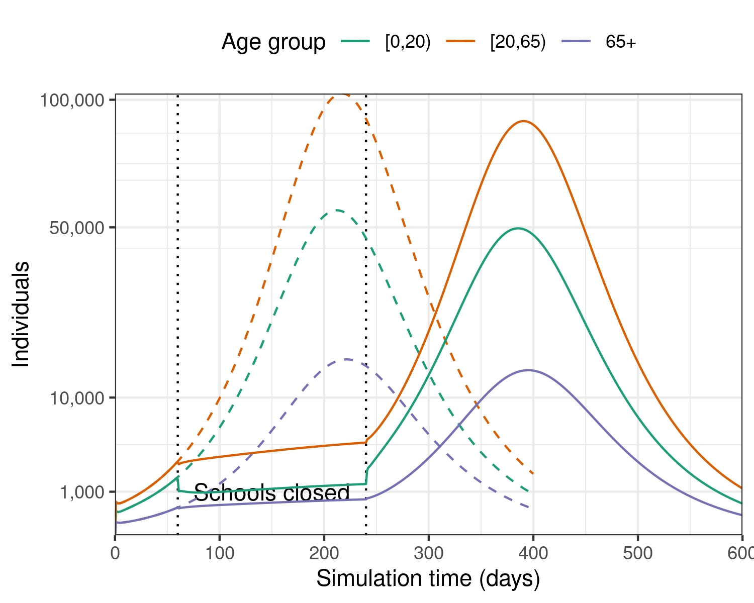

Epidemic model with an intervention that targets infections among children by closing schools for six months, thus reducing children's social contacts.

Figure 2: Epidemic model with an intervention that targets infections among children by closing schools for six months, thus reducing children’s social contacts.

In the school closures only scenario, the epidemic would continue for approximately 600 days, or more than one and a half years, with more than 10,000 daily new infections for over one year.

In this scenario, the epidemic is expected to have a final size of around 22 million individuals infected overall.

Workplace closures

General workplace closures are a broad-based measure aimed at reducing infections among all working age adults.

We shall prepare an intervention that simulates the effect of closing workplaces in addition to closing schools, and we assume that this reduces the contacts of the age group 20 – 65 by 30%, and the contacts of all other age groups by only 1% (we assume that individuals in other age groups are not meeting many individuals in workplaces).

This intervention is assumed to last 60 days, beginning from the 80th day of the outbreak — this simulates a situation in which policymakers decide to close workplaces three weeks after deciding to close schools, and in which they choose not to keep workplaces closed for as long (2 months or 60 days vs. 6 months or 180 days for school closures).

Code

# prepare an intervention which mostly affects adults 20 -- 65
intervention_duration <- 60
close_workplaces <- intervention(
  name = "Workplace closure",
  type = "contacts",
  time_begin = 80,
  time_end = 80 + intervention_duration,
  reduction = matrix(c(0.01, 0.3, 0.01))
)

# examine the intervention object
close_workplaces
#> 
#>  Intervention name: 
#>  Begins at: 
#> [1] 80
#> 
#>  Ends at: 
#> [1] 140
#> 
#>  Reduction: 
#>              Interv. 1
#> Demo. grp. 1      0.01
#> Demo. grp. 2      0.30
#> Demo. grp. 3      0.01

Combining interventions

We can use the c() function to combine two intervention objects into a single intervention that accommodates the effect of both interventions. This multiple intervention can then be passed — as a single intervention object — to an epidemic model in model_default().

When an intervention object is made up of multiple interventions the first intervention to be specified is treated as the baseline intervention, with an age-specific effect on reducing contacts during its duration of effect.

All further interventions are assumed to be additional percentage point increases on the effect of any active interventions.

Code

# combine interventions using `c()`
combined_interventions <- c(
  close_schools, close_workplaces
)

# visualise the combined intervention object
combined_interventions
#> 
#>  Intervention name: 
#>  Begins at: 
#>      npi_1 npi_2
#> [1,]    60    80
#> 
#>  Ends at: 
#>      npi_1 npi_2
#> [1,]   240   140
#> 
#>  Reduction: 
#>              Interv. 1 Interv. 2
#> Demo. grp. 1      0.30      0.01
#> Demo. grp. 2      0.01      0.30
#> Demo. grp. 3      0.01      0.01

We can combine any number of intervention objects into a single intervention object to be passed to model_default(). The cumulative effect of the interventions is handled automatically by the C++ code underlying epidemics.
Remember that two multiple interventions can also be combined using c(). It is important to be careful when doing this and make sure that only the interventions you intend to combine are concatenated together. For example, c(combined_interventions, combined_interventions) is valid, and would effectively double the effect of school and workplace closures in the example.

We simulate an epidemic using the model_default() function, calling the default model outlined in the “Get started vignette”.

We simulate the epidemic for 600 days.

Code

# get data from an epidemic model with both interventions
data_combined <- model_default(
  population = uk_population,
  intervention = list(contacts = combined_interventions),
  time_end = 600, increment = 1.0
)

# get data on new infections
data_infections <- new_infections(data_combined, by_group = TRUE)

Code

plot_intervention_cases <-
  ggplot() +
  geom_vline(
    xintercept = c(
      close_schools$time_begin,
      close_schools$time_end
    ),
    linetype = "dotted"
  ) +
  geom_vline(
    xintercept = c(
      close_workplaces$time_begin,
      close_workplaces$time_end
    ),
    colour = "red",
    linetype = "dotted"
  ) +
  annotate(
    geom = "text",
    x = mean(c(close_schools$time_begin, close_schools$time_end)),
    y = 50000,
    label = "Schools closed"
  ) +
  annotate(
    geom = "text",
    x = mean(c(
      close_workplaces$time_begin,
      close_workplaces$time_end
    )),
    y = 30000,
    colour = "red",
    label = "Workplaces\nclosed"
  ) +
  geom_line(
    data = data_baseline_infections,
    aes(time, new_infections, colour = demography_group),
    linetype = "dashed"
  ) +
  geom_line(
    data = data_infections,
    aes(time, new_infections, colour = demography_group),
    linetype = "solid"
  ) +
  scale_y_sqrt(
    labels = scales::comma,
    breaks = c(10^seq(3, 5), 5e4)
  ) +
  scale_colour_brewer(
    palette = "Dark2",
    name = "Age group"
  ) +
  coord_cartesian(
    expand = FALSE
  ) +
  theme_bw() +
  theme(
    legend.position = "top"
  ) +
  labs(
    x = "Simulation time (days)",
    linetype = "Compartment",
    y = "Individuals"
  )

plot_intervention_cases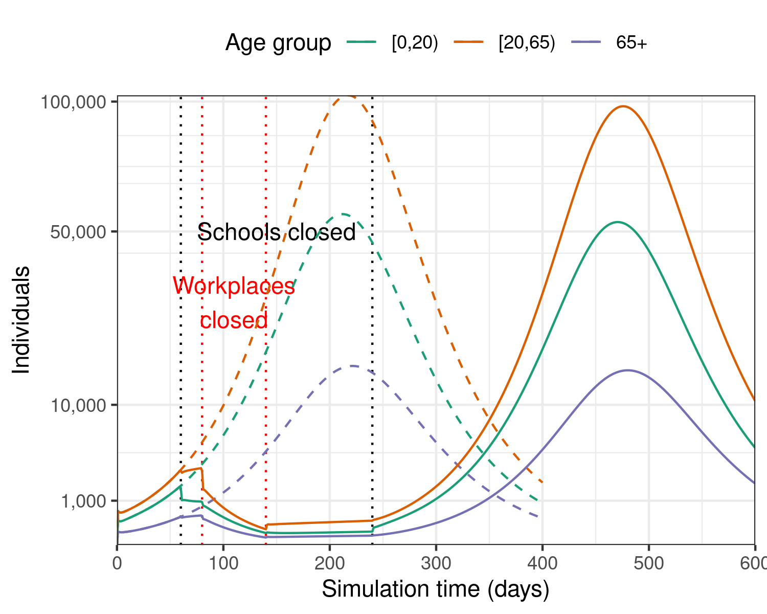

Epidemic model with two overlapping interventions in the early phase of the outbreak: school closures that target infections among younger people, and workplace closures which target infections among working-age adults.

Figure 3: Epidemic model with two overlapping interventions in the early phase of the outbreak: school closures that target infections among younger people, and workplace closures which target infections among working-age adults.

In this scenario with school closures for 6 months as well as workplace closures for 2 months, the epidemic would still continue for approximately 600 days, or more than one and a half years, but the number of days with 10,000 or more daily cases is reduced, and these typically occur once the intervention on workplaces is lifted.

In this scenario, the epidemic is expected to have a final size of around 22 million individuals infected overall — this is similar to the school closures only intervention.

There is a distinct peak new infections once schools are simulated to re-open, with nearly 100,000 new infections on some days.

Re-applying workplace closures

In the scenario with combined interventions, daily new infections are forecast to exceed 50,000 on the 397th day of the epidemic.

In this final example, we simulate re-implementing two months of workplace closures, but not school closures, to reduce infections.

Code

# log the date that cases exceed 50000 daily
start_date <- min(
  which(
    new_infections(data_combined, by_group = FALSE)[, new_infections > 50000]
  )
)

# create a new workplace closures object
workplace_closures_2 <- intervention(
  type = "contacts",
  time_begin = start_date,
  time_end = start_date + 60,
  reduction = matrix(c(0.01, 0.3, 0.01))
)

Combine the multiple interventions object with two interventions with the third intervention.

Code

combined_interventions <- c(combined_interventions, workplace_closures_2)

We simulate an epidemic using the model_default() function for 600 days as before.

Code

# get data from an epidemic model with both interventions
data_combined <- model_default(
  population = uk_population,
  intervention = list(contacts = combined_interventions),
  time_end = 600, increment = 1.0
)

# get data on new infections
data_infections <- new_infections(data_combined, by_group = TRUE)

Code

plot_three_interventions <-
  ggplot() +
  geom_vline(
    xintercept = c(
      close_schools$time_begin,
      close_schools$time_end
    ),
    linetype = "dotted"
  ) +
  geom_vline(
    xintercept = c(
      close_workplaces$time_begin,
      close_workplaces$time_end,
      workplace_closures_2$time_begin,
      workplace_closures_2$time_end
    ),
    colour = "red",
    linetype = "dotted"
  ) +
  annotate(
    geom = "text",
    x = mean(c(close_schools$time_begin, close_schools$time_end)),
    y = 50000,
    label = "Schools closed"
  ) +
  annotate(
    geom = "text",
    x = c(
      mean(
        c(close_workplaces$time_begin, close_workplaces$time_end)
      ),
      mean(c(workplace_closures_2$time_begin, workplace_closures_2$time_end))
    ),
    y = 30000,
    colour = "red",
    label = c("Workplaces\nclosed", "Workplaces\nclosed")
  ) +
  geom_line(
    data = data_baseline_infections,
    aes(time, new_infections, colour = demography_group),
    linetype = "dashed"
  ) +
  geom_line(
    data = data_infections,
    aes(time, new_infections, colour = demography_group),
    linetype = "solid"
  ) +
  scale_y_sqrt(
    labels = scales::comma,
    breaks = c(10^seq(3, 5), 5e4)
  ) +
  scale_colour_brewer(
    palette = "Dark2",
    name = "Age group"
  ) +
  coord_cartesian(
    expand = FALSE
  ) +
  theme_bw() +
  theme(
    legend.position = "top"
  ) +
  labs(
    x = "Simulation time (days)",
    linetype = "Compartment",
    y = "Individuals"
  )

plot_three_interventions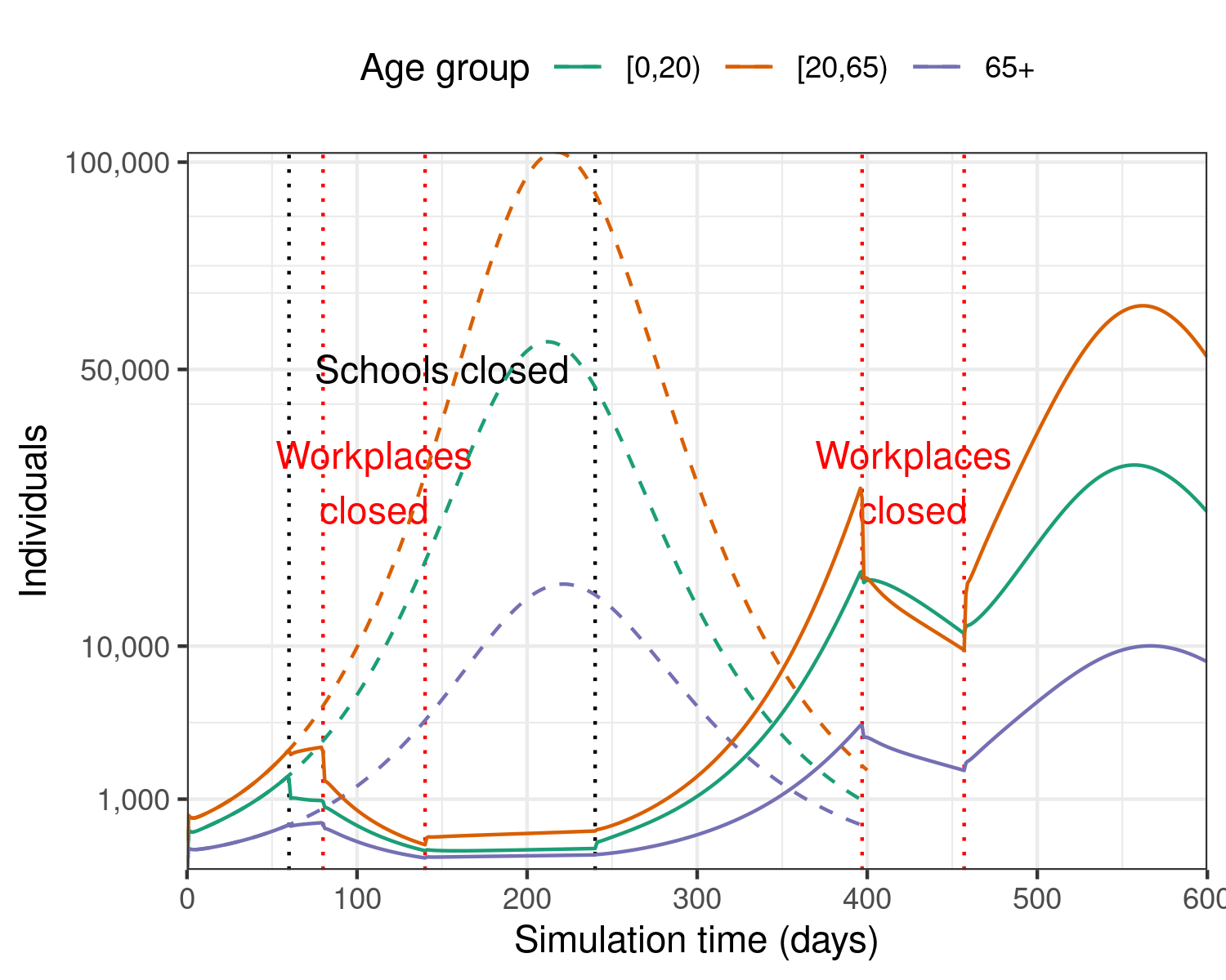

Figure 4: Epidemic model with two initial, overlapping interventions on schools and workplaces, followed by a later intervention on workplaces.

In this scenario with school closures for 6 months as well as two phases of workplace closures for 2 months each, the epidemic would continue for over 600 days, or more than one and a half years, but the number of days with 10,000 or more daily cases would be reduced, and these typically occur once the interventions on workplaces are lifted — this is similar to the previous example.

In this scenario, the epidemic is expected to have a final size of around 15 million individuals infected overall — this is lower than the previous examples.