Simulate Epidemic Attack Rates with Heterogeneous Social Contacts
Author
Adam Kucharski
Published
June 8, 2026
What do we have?
Basic reproduction number.
Social contact survey and demography data of Country in the POLYMOD study or Social contact data repository.
Susceptibility groups.
Probability of infection in demographic and susceptibility groups.
Steps in code
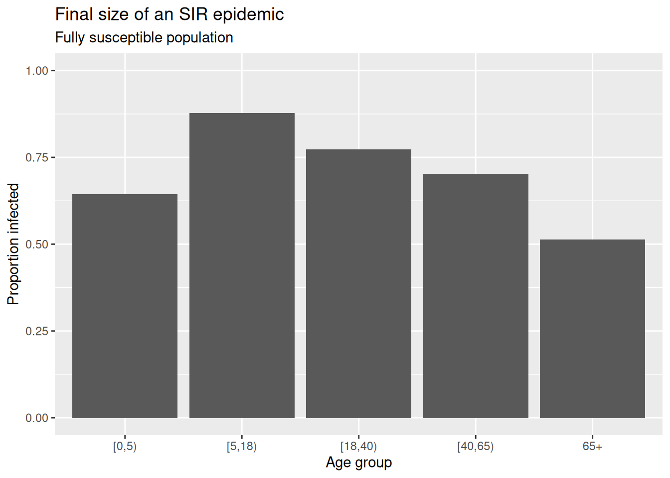
# Load packageslibrary(finalsize)library(socialmixr)library(tidyverse)# Simple quick calculation with homogenous mixing -------------------------------------------r0_input<-2finalsize::final_size(r0 =r0_input)#> demo_grp susc_grp susceptibility p_infected#> 1 demo_grp_1 susc_grp_1 1 0.7968124# Set up the transmission model -------------------------------------------# load contact and population data from socialmixr::polymodpolymod<-socialmixr::polymodcontact_data<-socialmixr::contact_matrix(polymod, countries ="United Kingdom", age.limits =c(0, 5, 18, 40, 65), symmetric =TRUE)# prepare contact matrix and demography vector for use in modelcontact_matrix<-t(contact_data$matrix)# transpose so R0 calculated correctly inside modeldemography_vector<-contact_data$demography$populationnames(demography_vector)<-rownames(contact_matrix)# scale the contact matrix so the largest eigenvalue is 1.0# this is to ensure that the overall epidemic dynamics correctly reflect# the assumed value of R0contact_matrix<-contact_matrix/max(Re(eigen(contact_matrix)$values))# divide each row of the contact matrix by the corresponding demography# this reflects the assumption that each individual in group {j} make contacts# at random with individuals in group {i}contact_matrix<-contact_matrix/demography_vectorn_demo_grps<-length(demography_vector)# all individuals are equally and highly susceptiblen_susc_groups<-1Lsusc_guess<-1.0susc_uniform<-matrix( data =susc_guess, nrow =n_demo_grps, ncol =n_susc_groups)# Final size calculations also need to know the proportion of each demographic group {𝑖} # that falls into the susceptibility group {𝑗}. This distribution of age groups into # susceptibility groups can be represented by the demography-susceptibility distribution matrix.p_susc_uniform<-matrix( data =1.0, nrow =n_demo_grps, ncol =n_susc_groups)output<-finalsize::final_size( r0 =r0_input, contact_matrix =contact_matrix, demography_vector =demography_vector, susceptibility =susc_uniform, p_susceptibility =p_susc_uniform)output#> demo_grp susc_grp susceptibility p_infected#> 1 [0,5) susc_grp_1 1 0.6434899#> 2 [5,18) susc_grp_1 1 0.8777478#> 3 [18,40) susc_grp_1 1 0.7723371#> 4 [40,65) susc_grp_1 1 0.7023265#> 5 [65,Inf) susc_grp_1 1 0.5131873output%>%mutate(demo_grp =as_factor(demo_grp))%>%ggplot(aes(x =demo_grp, y =p_infected))+geom_col()+ylim(0,1)+labs( x ="Age group", y ="Proportion infected", title ="Final size of an SIR epidemic", subtitle ="Fully susceptible population")
Steps in detail
This assume equal probability of infection in demographic and susceptibility groups.
Please note that the code assumes the necessary packages are already installed. If they are not, you can install them using first the install.packages("pak") function and then the pak::pak() function for both packages in CRAN or GitHub before loading them with library().