Populations are often heterogeneous in their social contact patterns. Such heterogeneity is often age-dependent and varies between age groups, and can strongly influence epidemic dynamics if the outbreak primarily circulates in a particular age group. This heterogeneity can be incorporated into final size calculations (Miller 2012), and is implemented in finalsize.
New to finalsize? It may help to read the “Get started” vignette first!
Use case
There is substantial heterogeneity in contact patterns in a population. We want to know how this heterogeneity could affect the final size of the epidemic.
What we have
- An estimate of the infection’s basic reproduction number \(R_0\);
- An estimate of the distribution of the population in different demographic groups (typically age groups);
- An estimate of the contacts between individuals of different demographic groups; and
- An estimate of the susceptibility of each demographic group to the infection.
What we assume
- That the infection dynamics can be captured using a Susceptible-Infectious-Recovered (SIR) or Susceptible-Exposed-Infectious-Recovered (SEIR) model, where individuals who have been infected acquire immunity against subsequent infection, at least for the remaining duration of the epidemic.
Defining a value for \(R_0\)
A number of statistical methods can be used to estimate the \(R_0\) of an epidemic in its early stages from available data. These are not discussed here, but some examples are given in the episoap package.
Instead, this example considers a infection with an \(R_0\) of 1.5, similar to that which could potentially be observed for pandemic influenza.
Code
# define r0 as 1.5
r0 <- 1.5
Heterogeneous social mixing
The social contact data used in this example illustrate an important way in which populations may be heterogeneous: the various age groups can have substantially different patterns of social contacts, and hence different probabilities of acquiring and transmitting infection during an epidemic.
The method implemented in finalsize accounts for this heterogeneity. Other forms of population heterogeneity are covered in the “Heterogeneous susceptibility” vignette.
Getting and preparing contact and demography data
This example uses social contact data from the POLYMOD project (Mossong et al. 2008) to estimate the final size of an epidemic in the U.K. These data are provided with the socialmixr package.
The contact data are divided into five age groups: 0 – 4, 5 – 17, 18 – 39, 40 – 64, and 65 and over, specified using the age.limits argument in socialmixr::contact_matrix().
The symmetric = TRUE argument to socialmixr::contact_matrix() returns a symmetric contact matrix, so that the contacts reported by group \(\{i\}\) of individuals from group \(\{j\}\) are the same as those reported by group \(\{j\}\) of group \(\{i\}\).
The demographic data — the number of individuals in each age group — is also available through socialmixr::contact_matrix().
Code
# get UK polymod data
polymod <- socialmixr::polymod
contact_data <- socialmixr::contact_matrix(
  polymod,
  countries = "United Kingdom",
  age.limits = c(0, 5, 18, 40, 65),
  symmetric = TRUE
)

# view the elements of the contact data list
# the contact matrix
contact_data$matrix
#>       contact.age.group
#>            [0,5)   [5,18)  [18,40)  [40,65)       65+
#>   [1,] 1.9157895 1.467205 3.278803 1.559611 0.3658614
#>   [2,] 0.5191021 8.858736 3.421566 2.616146 0.6260247
#>   [3,] 0.6252718 1.844236 5.440972 3.492124 0.8092367
#>   [4,] 0.2792593 1.324010 3.278895 4.178218 1.2380907
#>   [5,] 0.1306272 0.631752 1.515092 2.468756 1.7142857

# the demography data
contact_data$demography
#>    age.group population proportion  year
#>       <char>      <num>      <num> <int>
#> 1:     [0,5)    3453670 0.05728738  2005
#> 2:    [5,18)    9761554 0.16191873  2005
#> 3:   [18,40)   18110368 0.30040378  2005
#> 4:   [40,65)   19288101 0.31993930  2005
#> 5:       65+    9673058 0.16045081  2005

# get the contact matrix and demography data
contact_matrix <- t(contact_data$matrix)
demography_vector <- contact_data$demography$population
demography_data <- contact_data$demography

# scale the contact matrix so the largest eigenvalue is 1.0
# this is to ensure that the overall epidemic dynamics correctly reflect
# the assumed value of R0
contact_matrix <- contact_matrix / max(Re(eigen(contact_matrix)$values))

# divide each row of the contact matrix by the corresponding demography
# this reflects the assumption that each individual in group {j} make contacts
# at random with individuals in group {i}
contact_matrix <- contact_matrix / demography_vector

n_demo_grps <- length(demography_vector)
Population susceptibility
As a starting scenario, consider a novel pathogen where all age groups have a similar, high susceptibility to infection. This means it is assumed that all individuals fall into a single category: fully susceptible.
Full uniform susceptibility can be modelled as a matrix with values of 1.0, with as many rows as there are demographic groups. The matrix has a single column, representing the single susceptibility group to which all individuals belong.
Code
# all individuals are equally and highly susceptible
n_susc_groups <- 1L
susc_guess <- 1.0
Code
susc_uniform <- matrix(
  data = susc_guess,
  nrow = n_demo_grps,
  ncol = n_susc_groups
)
Final size calculations also need to know the proportion of each demographic group \(\{i\}\) that falls into the susceptibility group \(\{j\}\). This distribution of age groups into susceptibility groups can be represented by the demography-susceptibility distribution matrix.
Since all individuals in each age group have the same susceptibility, there is no variation within age groups. Consequently, all individuals in each age group are assumed to be fully susceptible. This can be represented as a single-column matrix, with as many rows as age groups, and as many columns as susceptibility groups.
In this example, the matrix p_susc_uniform has 5 rows, one for each age group, and only one column, for the single high susceptibility group that holds all individuals.
Code
p_susc_uniform <- matrix(
  data = 1.0,
  nrow = n_demo_grps,
  ncol = n_susc_groups
)
Why susceptibility and p_susceptibility are matrices
This example models susceptibility (susc_uniform) and the demography-in-susceptibility (p_susc_uniform) as matrices rather than vectors. This is because a single susceptibility group is a special case of the general final size equation.
finalsize supports multiple susceptibility groups (this will be covered later), and these are more easily represented as a matrix, the susceptibility matrix.
Each element \(\{i, j\}\) in this matrix represents the susceptibility of individuals in demographic group \(\{i\}\), and susceptibility group \(\{j\}\).
In this example, all individuals are equally susceptible to infection, and thus the susceptibility matrix (susc_uniform) has only a single column with identical values.
Consequently, the demography-susceptibility distribution matrix (p_susc_uniform) has the same dimensions, and all of its values are 1.0.
See the “Heterogeneous susceptibility” example for more on cases where susceptibility varies within age groups.
Running final_size
The final size of the epidemic in the population can then be calculated using the only function in the package, final_size(). This example allows the function to fall back on the default options for the arguments solver ("iterative") and control (an empty list).
Code
# calculate final size
final_size_data <- final_size(
  r0 = r0,
  contact_matrix = contact_matrix,
  demography_vector = demography_vector,
  susceptibility = susc_uniform,
  p_susceptibility = p_susc_uniform
)

# view the output data frame
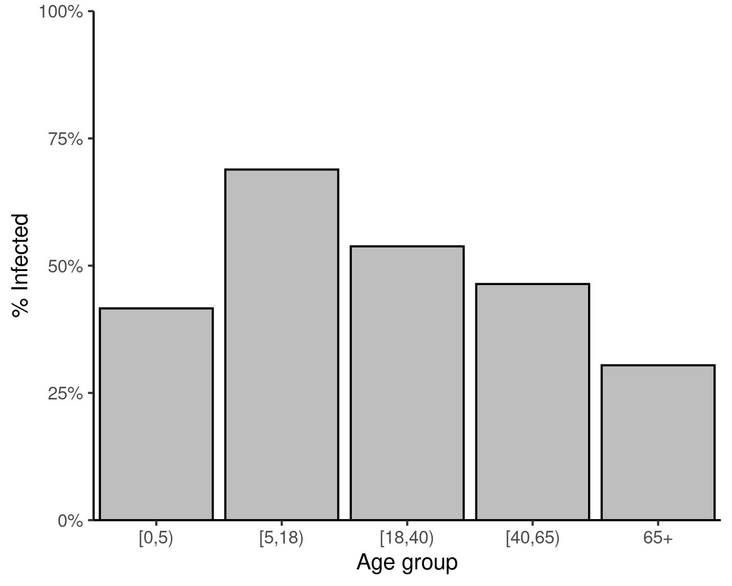
final_size_data
#>   demo_grp   susc_grp susceptibility p_infected
#> 1    [0,5) susc_grp_1              1  0.4160682
#> 2   [5,18) susc_grp_1              1  0.6888703
#> 3  [18,40) susc_grp_1              1  0.5379381
#> 4  [40,65) susc_grp_1              1  0.4639496
#> 5      65+ susc_grp_1              1  0.3042623
Visualise final sizes
Code
# order demographic groups as factors
final_size_data$demo_grp <- factor(
  final_size_data$demo_grp,
  levels = demography_data$age.group
)
Code
# plot data
ggplot(final_size_data) +
  geom_col(
    aes(
      demo_grp, p_infected
    ),
    colour = "black", fill = "grey"
  ) +
  scale_y_continuous(
    labels = scales::percent,
    limits = c(0, 1)
  ) +
  expand_limits(
    x = c(0.5, nrow(final_size_data) + 0.5)
  ) +
  theme_classic() +
  coord_cartesian(
    expand = FALSE
  ) +
  labs(
    x = "Age group",
    y = "% Infected"
  )
Figure 1: Final size of an SIR epidemic in each age group. The final size is the cumulative number of infections in each age group over the course of the epidemic, expressed as a proportion of the respective age group.
Final size proportions to counts
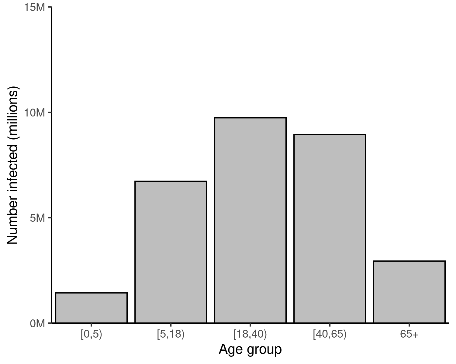
finalsize returns the proportion of each age (and susceptibility) group infected in an epidemic outbreak. The final counts of individuals infected can be visualised as well, by multiplying the final proportion of each age group infected with the total number of individuals in that group.
The example below show how this can be done.
Code
# prepare demography data
demography_data <- contact_data$demography

# merge final size counts with demography vector
final_size_data <- merge(
  final_size_data,
  demography_data,
  by.x = "demo_grp",
  by.y = "age.group"
)

# reset age group order
final_size_data$demo_grp <- factor(
  final_size_data$demo_grp,
  levels = contact_data$demography$age.group
)

# multiply counts with proportion infected
final_size_data$n_infected <- final_size_data$p_infected *
  final_size_data$population
Code
ggplot(final_size_data) +
  geom_col(
    aes(
      x = demo_grp, y = n_infected
    ),
    fill = "grey", col = "black"
  ) +
  expand_limits(
    x = c(0.5, nrow(final_size_data) + 0.5)
  ) +
  scale_y_continuous(
    labels = scales::comma_format(
      scale = 1e-6, suffix = "M"
    ),
    limits = c(0, 15e6)
  ) +
  theme_classic() +
  coord_cartesian(
    expand = FALSE
  ) +
  labs(
    x = "Age group",
    y = "Number infected (millions)"
  )
Figure 2: Final size of an epidemic outbreak in a population, for different values of infection \(R_0\). Converting the final size proportions in each age group to counts shows that individuals aged 18 – 64 make up the bulk of cases in this scenario. This may be attributed to this being both the largest age range in the analysis (more years in this range than any other), and because more people fall into this wide range than others. Contrast this figure with the one above, in which similar proportions of each age group are infected.