Introduction to delays
Last updated on 2026-06-14 | Edit this page
Overview
Questions
- How to fit a probability distribution to delay data?
- How to interpret distribution parameters?
- How to access distribution parameters from fitting objects
Objectives
- Fit a probability distribution to data using fitdistrplus
- Extract a single column using
pull(), dollar sign$, or square brackets[].
Introduction
Delays are key for downstream task in outbreak analytics. To estimate the outbreak severity, we need to assume a known delay from onset to death. To quantify transmission, we need to consider delays from the moment of infection to the time of data collection. In order to account for epidemiological delays when estimating indicators of severity or transmission, in our analysis we need to input delays as Probability Distributions.
Let’s start by loading the package dplyr to manipulate
data. We’ll use the pipe %>% to connect some of their
functions, including others from the package ggplot2, so
let’s call to the package tidyverse that loads them all.
We will also use fitdistrplus to fit probability
distributions to delays:
R
# Load packages
library(tidyverse) # loads dplyr, the pipe, and ggplot2
library(fitdistrplus)
The double-colon
The double-colon :: in R let you call a specific
function from a package without loading the entire package into the
current environment.
For example, dplyr::filter(data, condition) uses
filter() from the dplyr package.
This helps us remember package functions and avoid namespace conflicts.
Fit a probability distribution to delays
We fit a probability distribution to data (like delays) to make inferences about it. These inferences can be useful for Public health interventions and decision making. For example:
From the incubation period distribution we can inform the length of active monitoring or quarantine. We can infer the time by which 99% of infected individuals are expected to show symptoms (Lauer et al., 2020).
From the serial interval distribution we can optimize contact tracing. We can evaluate the need to expand the number of days pre-onset to consider in the contact tracing to include more backwards contacts (Claire Blackmore, 2021; Davis et al., 2020).
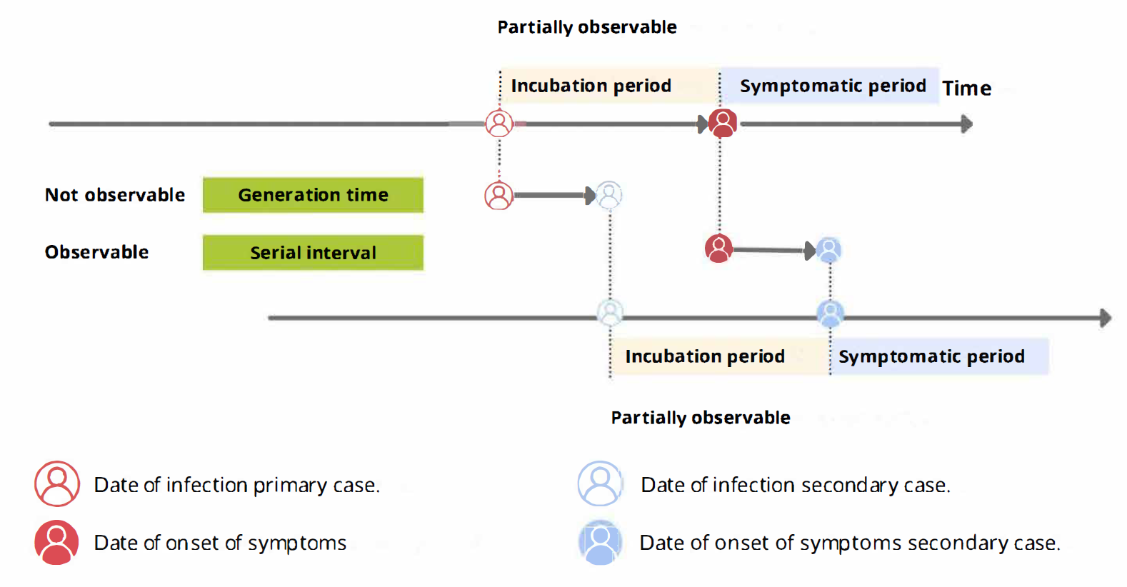
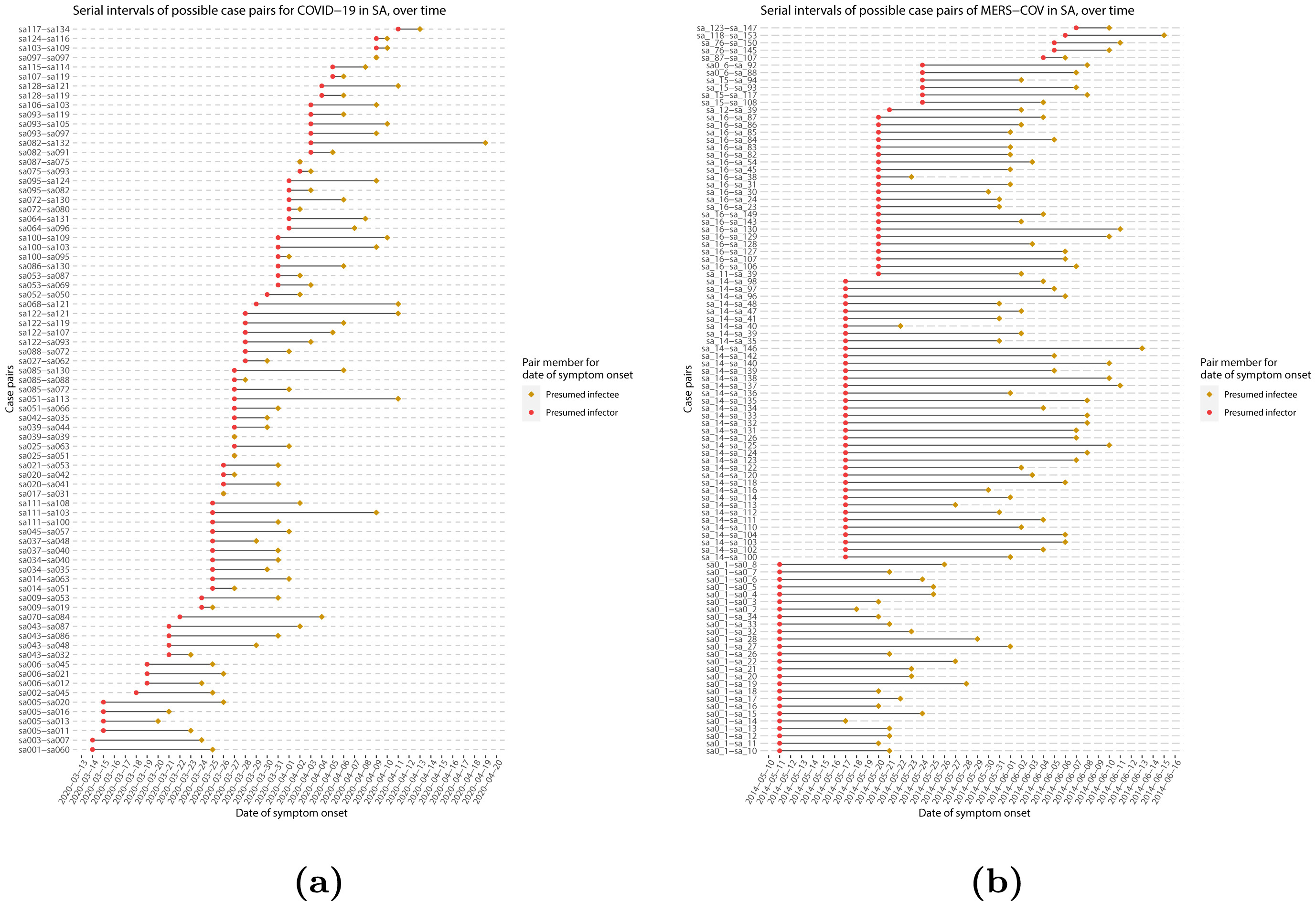
From time periods to probability distributions
When we calculate the serial interval, we see that not all case pairs have the same time length. We will observe this variability for any case pair and individual time period.
To summarise these data from individual and pair time periods, we can find the statistical distributions that best fit the data (McFarland et al., 2023).
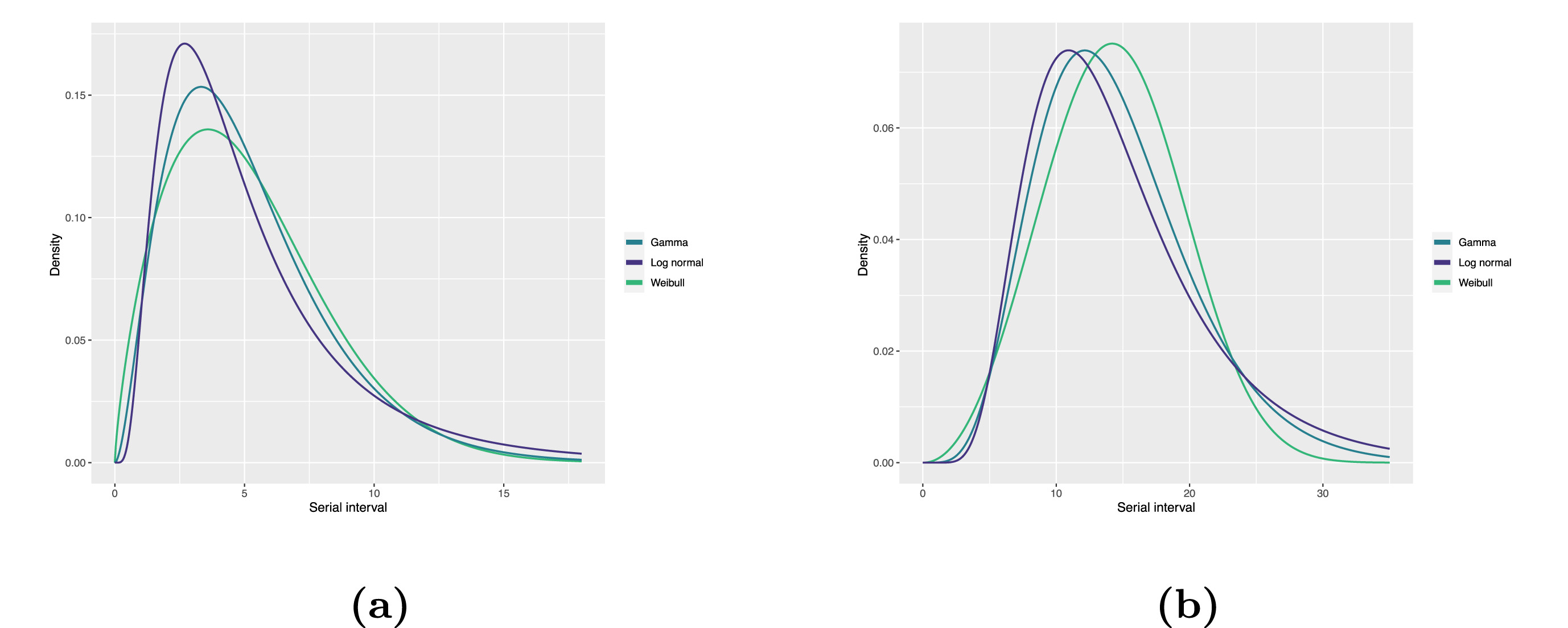
Statistical distributions are summarised in terms of their summary statistics like the location (mean and percentiles) and spread (variance or standard deviation) of the distribution, or with their distribution parameters that inform about the form (shape and rate/scale) of the distribution. These estimated values can be reported with their uncertainty (95% confidence intervals).
| Gamma | mean | shape | rate/scale |
|---|---|---|---|
| MERS-CoV | 14.13(13.9–14.7) | 6.31(4.88–8.52) | 0.43(0.33–0.60) |
| COVID-19 | 5.1(5.0–5.5) | 2.77(2.09–3.88) | 0.53(0.38–0.76) |
| Weibull | mean | shape | rate/scale |
|---|---|---|---|
| MERS-CoV | 14.2(13.3–15.2) | 3.07(2.64–3.63) | 16.1(15.0–17.1) |
| COVID-19 | 5.2(4.6–5.9) | 1.74(1.46–2.11) | 5.83(5.08–6.67) |
| Log normal | mean | mean-log | sd-log |
|---|---|---|---|
| MERS-CoV | 14.08(13.1–15.2) | 2.58(2.50–2.68) | 0.44(0.39–0.5) |
| COVID-19 | 5.2(4.2–6.5) | 1.45(1.31–1.61) | 0.63(0.54–0.74) |
To illustrate this, let’s continue with the same line list from the previous episode:
R
# Read data
# e.g.: if path to file is data/linelist.csv then:
cases <- readr::read_csv(
  here::here("data", "linelist.csv")
)
From the cases object we can use:
-
dplyr::mutate()to transform thereporting_delayclass object from<time>to<numeric>, -
dplyr::filter()to keep the positive values, -
dplyr::pull()to extract a single column, -
fitdistrplus::fitdist()to fit a probability distribution using Maximum Likelihood. We can test distributions like the Log Normal ("lnorm"),"gamma", or"weibull".
R
cases %>%
dplyr::select(case_id, date_of_onset, date_of_hospitalisation) %>%
dplyr::mutate(reporting_delay = date_of_hospitalisation - date_of_onset) %>%
dplyr::mutate(reporting_delay_num = as.numeric(reporting_delay)) %>%
dplyr::filter(reporting_delay_num > 0) %>%
dplyr::pull(reporting_delay_num) %>%
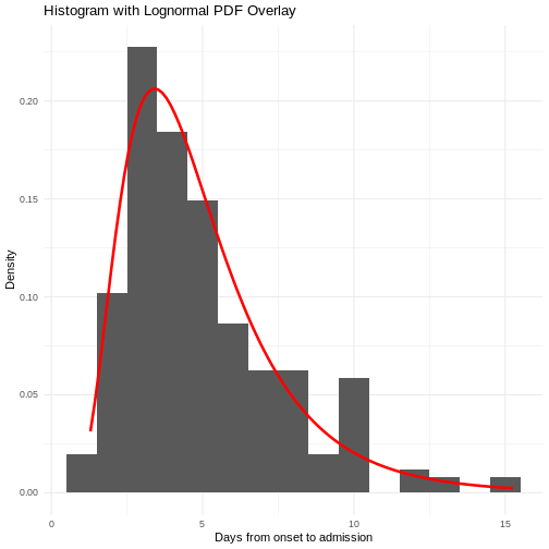
fitdistrplus::fitdist(distr = "lnorm")
OUTPUT
Fitting of the distribution ' lnorm ' by maximum likelihood
Parameters:
         estimate Std. Error
meanlog 1.0488098 0.06866105
sdlog   0.8465102 0.04855039
Use summary() to find goodness-of-fit statistics from
the Maximum likelihood. Use plot() to visualize the fitted
density function and other quality control plots. To compare multiple
distributions you can use superspreading::ic_tbl().
We’ll explore that package later!
Now we can do inferences from the probability distribution fitted to the epidemiological delay! Want to learn how? Read the “Show details” :)
Making inferences from probability distributions
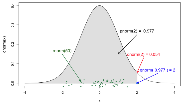
From probability distributions we can infer estimates like cumulative probability, maximum values, or generate random values. We can access to them using R probability functions.
We recommend you read the definitions of the R probability functions for the Normal distribution. From it we can relate with any other family of statistical distributions!
Each probability distribution has a unique set of
parameters and probability functions.
Read the Distributions
in the stats package or ?stats::Distributions to find
the ones available in R.
For example, assuming that the reporting delay follows a Log
Normal distribution, we can use plnorm() to
calculate the probability of observing a reporting delay of 14 days or
less:
R
plnorm(q = 14, meanlog = 1.0488098, sdlog = 0.8465102)
OUTPUT
[1] 0.9698499Or the amount of time by which 99% of symptomatic individuals are expected to be reported in the hospitalization record:
R
qlnorm(p = 0.99, meanlog = 1.0488098, sdlog = 0.8465102)
OUTPUT
[1] 20.45213You will find more examples of how to use delays for decision-making at the Use delay distributions in analysis at Tutorials Middle!
To interactively explore probability distributions, their parameters and access to their distribution functions, we suggest to explore a shinyapp called The Distribution Zoo: https://ben18785.shinyapps.io/distribution-zoo/
Let’s review some operators used until now:
- Assignment
<-assigns a value to a variable from right to left. - Double colon
::to call a function from a specific package. - Pipe
%>%to structure sequences of data operations left-to-right
We need to add two more to the list:
- Dollar sign
$ - Square brackets
[]
Last step is to access to this parameters. Most modeling outputs from
R functions will be stored as list class objects. In R, the
dollar sign operator $ is used to access elements (like
columns) within a data frame or list by name, allowing for easy
retrieval of specific components.
A code completion tip
If we write the square brackets [] next
to the object reporting_delay_fit$estimate[], within
[] we can use the Tab key ↹ for code
completion feature
This gives quick access to "meanlog" and
"sdlog". We invite you to try this out in code chunks and
the R console!
R
# 1. Place the cursor within the square brackets
# 2. Use the Tab key
# 3. Explore the completion list
# 4. Select for "meanlog" or "sdlog"
reporting_delay_fit$estimate[]
Estimating epidemiological delays is CHALLENGING!
Epidemiological delays need to account for biases like censoring, right truncation, or epidemic phase (Charniga et al., 2024).
Additionally, at the beginning of an outbreak, limited data or resources exist to perform this during a real-time analysis. Until we have more appropriate data for the specific disease and region of the ongoing outbreak, we can reuse delays from past outbreaks from the same pathogens or close in its phylogeny, independent of the area of origin.
Next step
In the following tutorial episodes, we will:
- Efficiently clean and produce epidemic curves to explore patterns of disease spread by different groups and time aggregates. Find more in Tutorials Early!
- Access to epidemiological delay distributions to estimate delay-adjusted transmission and severity metrics (e.g. reproduction number and case fatality risk). Find more in Tutorials Middle!
- Use parameter values like the basic reproduction number, and delays like the latent period and infectious period to simulate transmission trajectories and intervention scenarios. Find more in Tutorials Late!
Challenges
Challenge
Relevant delays when estimating transmission
Review the definition of the incubation period in our glossary page.
Calculate the summary statistics of the incubation period distribution observed in the line list.
Visualize the distribution of the incubation period from the line list.
Fit a log-normal distribution to get the probability distribution parameters of the the observed incubation period.
(Optional) Infer the time by which 99% of infected individuals are expected to show symptoms.
Calculate the summary statistics:
R
cases %>%
  dplyr::select(case_id, date_of_infection, date_of_onset) %>%
  dplyr::mutate(incubation_period = date_of_onset - date_of_infection) %>%
  skimr::skim(incubation_period)
| Name | Piped data |
| Number of rows | 166 |
| Number of columns | 4 |
| _______________________ | |
| Column type frequency: | |
| difftime | 1 |
| ________________________ | |
| Group variables | None |
Variable type: difftime
| skim_variable | n_missing | complete_rate | min | max | median | n_unique |
|---|---|---|---|---|---|---|
| incubation_period | 61 | 0.63 | 1 days | 37 days | 5 days | 25 |
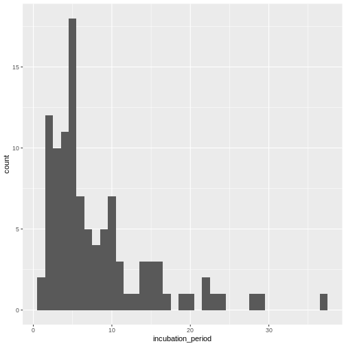
Visualize the distribution:
R
cases %>%
  dplyr::select(case_id, date_of_infection, date_of_onset) %>%
  dplyr::mutate(incubation_period = date_of_onset - date_of_infection) %>%
  ggplot(aes(x = incubation_period)) +
  geom_histogram(binwidth = 1)
Fit a log-normal distribution:
R
incubation_period_dist <- cases %>%
  dplyr::select(case_id, date_of_infection, date_of_onset) %>%
  dplyr::mutate(incubation_period = date_of_onset - date_of_infection) %>%
  mutate(incubation_period_num = as.numeric(incubation_period)) %>%
  filter(!is.na(incubation_period_num)) %>%
  pull(incubation_period_num) %>%
  fitdistrplus::fitdist(distr = "lnorm")

incubation_period_dist
OUTPUT
Fitting of the distribution ' lnorm ' by maximum likelihood
Parameters:
         estimate Std. Error
meanlog 1.8037993 0.07381350
sdlog   0.7563633 0.05219361
(Optional) Infer the time by which 99% of infected individuals are expected to show symptoms:
R
qlnorm(
  p = 0.99,
  meanlog = incubation_period_dist$estimate["meanlog"],
  sdlog = incubation_period_dist$estimate["sdlog"]
)
OUTPUT
[1] 35.28167With the distribution parameters of the incubation period we can infer the length of active monitoring or quarantine. Lauer et al., 2020 estimated the incubation period of Coronavirus Disease 2019 (COVID-19) from publicly reported confirmed cases.
- Epidemiological delays condition the estimation of indicators for severity or transmission.
- Fit probability distribution to delays to make inferences from them for decision-making.
- Fitting epidemiological delays need to account for biases like censoring, right truncation, or epidemic phase.
References
Cori, A. et al. (2019) Real-time outbreak analysis: Ebola as a case study - part 1 · Recon Learn, RECON learn. Available at: https://www.reconlearn.org/post/real-time-response-1 (Accessed: 06 November 2024).
Cori, A. et al. (2019) Real-time outbreak analysis: Ebola as a case study - part 2 · Recon Learn, RECON learn. Available at: https://www.reconlearn.org/post/real-time-response-2 (Accessed: 07 November 2024).