# Load packages
library(cleanepi)
library(linelist)
library(incidence2)
library(tidyverse)
# Read data
dat <- readRDS(system.file("extdata", "test_df.RDS", package = "cleanepi")) %>%
dplyr::as_tibble()
# View raw data
dat
#> # A tibble: 10 × 8
#> study_id event_name country_code country_name date.of.admission dateOfBirth
#> <chr> <chr> <int> <chr> <chr> <chr>
#> 1 PS001P2 day 0 2 Gambia 01/12/2020 06/01/1972
#> 2 PS002P2 day 0 2 Gambia 28/01/2021 02/20/1952
#> 3 PS004P2-1 day 0 2 Gambia 15/02/2021 06/15/1961
#> 4 PS003P2 day 0 2 Gambia 11/02/2021 11/11/1947
#> 5 P0005P2 day 0 2 Gambia 17/02/2021 09/26/2000
#> 6 PS006P2 day 0 2 Gambia 17/02/2021 -99
#> 7 PB500P2 day 0 2 Gambia 28/02/2021 11/03/1989
#> 8 PS008P2 day 0 2 Gambia 22/02/2021 10/05/1976
#> 9 PS010P2 day 0 2 Gambia 02/03/2021 09/23/1991
#> 10 PS011P2 day 0 2 Gambia 05/03/2021 02/08/1991
#> # ℹ 2 more variables: date_first_pcr_positive_test <chr>, sex <int>
# 1 Clean and standardize raw data
dat_clean <- dat %>%
# Standardize column names and dates
cleanepi::standardize_column_names() %>%
cleanepi::standardize_dates(
target_columns = c("date_of_birth","date_first_pcr_positive_test")
) %>%
# Replace from strings to a valid missing entry
cleanepi::replace_missing_values(
target_columns = "sex",
na_strings = "-99") %>%
# Calculate the age in 'years' and return the remainder in 'months'
cleanepi::timespan(
target_column = "date_of_birth",
end_date = Sys.Date(),
span_unit = "years",
span_column_name = "age_in_years",
span_remainder_unit = "months"
) %>%
# Select key variables
dplyr::select(
study_id,
sex,
date_first_pcr_positive_test,
date_of_birth,
age_in_years
) %>%
# Categorize the age numerical variable
dplyr::mutate(
age_category = base::cut(
x = age_in_years,
breaks = c(0,20,35,60,100), # replace with max value if known
include.lowest = TRUE,
right = FALSE
)
) %>%
dplyr::mutate(
sex = as.factor(sex)
)
# View cleaned data
dat_clean
#> # A tibble: 10 × 6
#> study_id sex date_first_pcr_posit…¹ date_of_birth age_in_years age_category
#> <chr> <fct> <date> <date> <dbl> <fct>
#> 1 PS001P2 1 2020-12-01 1972-01-06 54 [35,60)
#> 2 PS002P2 1 2021-01-01 1952-02-20 74 [60,100]
#> 3 PS004P2… <NA> 2021-02-11 1961-06-15 64 [60,100]
#> 4 PS003P2 1 2021-02-01 1947-11-11 78 [60,100]
#> 5 P0005P2 2 2021-02-16 2000-09-26 25 [20,35)
#> 6 PS006P2 2 2021-05-02 NA NA <NA>
#> 7 PB500P2 1 2021-02-19 1989-03-11 37 [35,60)
#> 8 PS008P2 2 2021-09-20 1976-05-10 50 [35,60)
#> 9 PS010P2 1 2021-02-26 1991-09-23 34 [20,35)
#> 10 PS011P2 2 2021-03-03 1991-08-02 34 [20,35)
#> # ℹ abbreviated name: ¹date_first_pcr_positive_test
# 2 Tag and validate linelist
dat_linelist <- dat_clean %>%
# Tag variables
linelist::make_linelist(
id = "study_id",
date_reporting = "date_first_pcr_positive_test",
gender = "sex",
age = "age_in_years",
age_group = "age_category", allow_extra = TRUE
) %>%
# Validate linelist
linelist::validate_linelist(
allow_extra = TRUE,
ref_types = linelist::tags_types(
age_group = c("factor"),
allow_extra = TRUE
)
) %>%
# Get tag and validated columns
linelist::tags_df()
# View tagged data (column names change)
dat_linelist
#> # A tibble: 10 × 5
#> id date_reporting gender age age_group
#> <chr> <date> <fct> <dbl> <fct>
#> 1 PS001P2 2020-12-01 1 54 [35,60)
#> 2 PS002P2 2021-01-01 1 74 [60,100]
#> 3 PS004P2-1 2021-02-11 <NA> 64 [60,100]
#> 4 PS003P2 2021-02-01 1 78 [60,100]
#> 5 P0005P2 2021-02-16 2 25 [20,35)
#> 6 PS006P2 2021-05-02 2 NA <NA>
#> 7 PB500P2 2021-02-19 1 37 [35,60)
#> 8 PS008P2 2021-09-20 2 50 [35,60)
#> 9 PS010P2 2021-02-26 1 34 [20,35)
#> 10 PS011P2 2021-03-03 2 34 [20,35)
# 3 Aggregate linelist to incidence
dat_incidence <- dat_linelist %>%
# Transform from individual-level to time-aggregate
incidence2::incidence(
date_index = "date_reporting", #"date_first_pcr_positive_test",
groups = "age_group", #"age_category", # change to sex, ...
interval = "month", # change to days, weeks, ...
# complete_dates = TRUE # relevant to downstream analysis [time-series data]
)
# View incidence data
dat_incidence
#> # incidence: 8 x 4
#> # count vars: date_reporting
#> # groups: age_group
#> date_index age_group count_variable count
#> <yrmon> <fct> <chr> <int>
#> 1 2020-Dec [35,60) date_reporting 1
#> 2 2021-Jan [60,100] date_reporting 1
#> 3 2021-Feb [20,35) date_reporting 2
#> 4 2021-Feb [35,60) date_reporting 1
#> 5 2021-Feb [60,100] date_reporting 2
#> 6 2021-Mar [20,35) date_reporting 1
#> 7 2021-May <NA> date_reporting 1
#> 8 2021-Sep [35,60) date_reporting 1
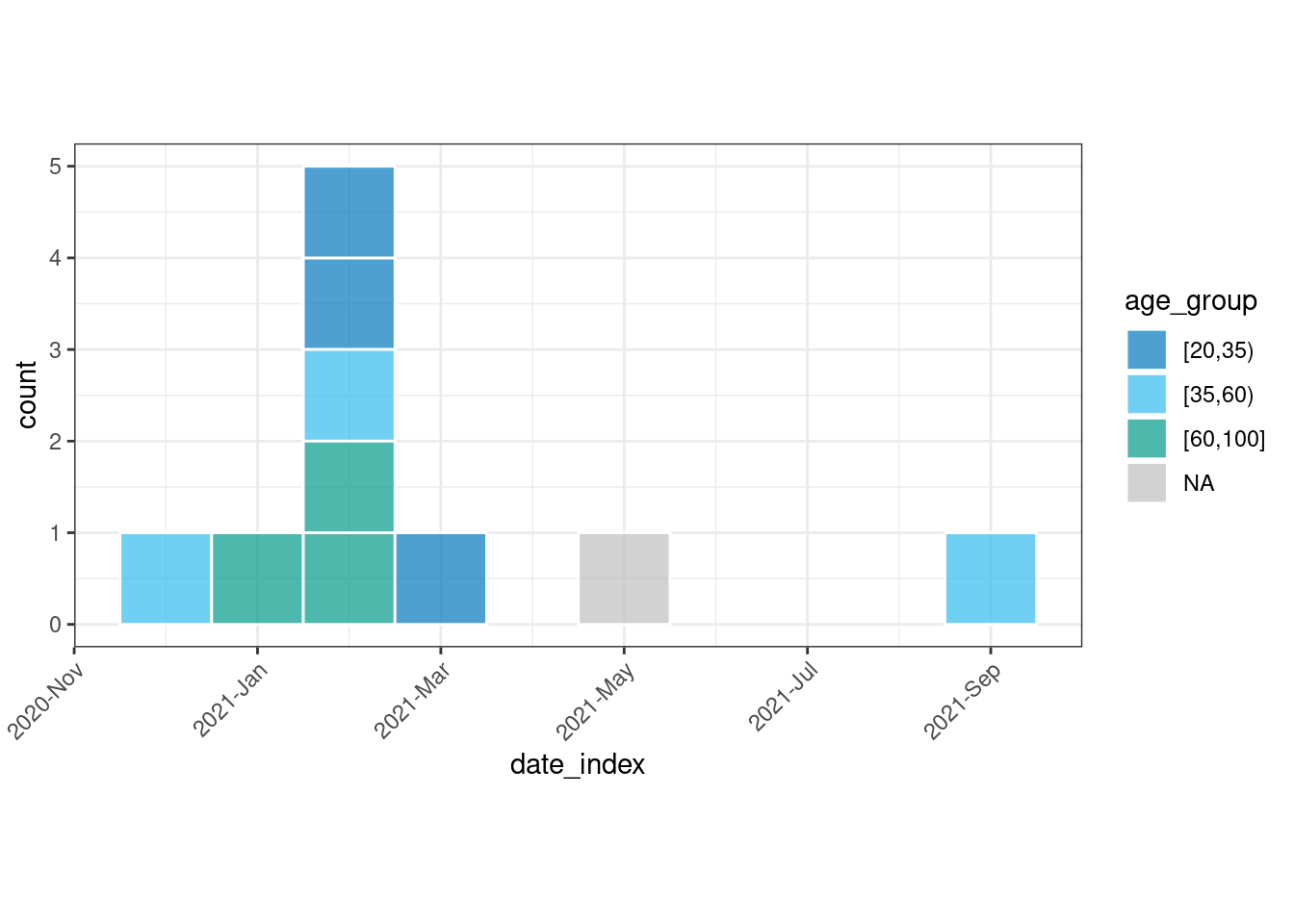
# Plot incidence data
dat_incidence %>%
plot(
fill = "age_group", # "age_category",
show_cases = TRUE, angle = 45, n_breaks = 5 # alternative options (vignette)
)