Simple analysis
Last updated on 2024-06-18 | Edit this page
Overview
Questions
- What is the growth rate of the epidemic?
- How to identify the peak time of an outbreak?
- How to compute moving average of cases?
Objectives
- Perform an early analysis of outbreak data
- Identify trends, exponential, doubling, and peak time
Introduction
Understanding the trend in case data is crucial for various purposes, such as forecasting future case counts, implementing public health interventions, and assessing the effectiveness of control measures. By analyzing the trend, policymakers and public health experts can make informed decisions to mitigate the spread of diseases and protect public health. This episode focuses on how to perform a simple early analysis on incidence data. It uses the same dataset of Covid-19 case data from England that utilized it in Aggregate and visualize episode.
The double-colon
The double-colon :: in R let you call a specific
function from a package without loading the entire package into the
current environment.
For example, dplyr::filter(data, condition) uses
filter() from the dplyr package.
This help us remember package functions and avoid namespace conflicts.
Simple model
Aggregated case data over a specific time unit, or incidence data,
typically represent the number of cases occurring within that time
frame. These data can often be assumed to follow either
Poisson distribution or a
negative binomial (NB) distribution, depending on the
specific characteristics of the data and the underlying processes
generating them. When analyzing such data, one common approach is to
examine the trend over time by computing the rate of change, which can
indicate whether there is exponential growth or decay in the number of
cases. Exponential growth implies that the number of cases is increasing
at an accelerating rate over time, while exponential decay suggests that
the number of cases is decreasing at a decelerating rate.
The i2extras package provides methods for modelling the
trend in case data, calculating moving averages, and exponential growth
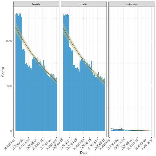
or decay rate. The code chunk below computes the Covid-19 trend in UK
within first 3 months using negative binomial distribution.
R
# load packages which provides methods for modeling
library("i2extras")
library("incidence2")

# read data from {outbreaks} package
covid19_eng_case_data <- outbreaks::covid19_england_nhscalls_2020

# subset the covid19_eng_case_data to include only the first 3 months of data
df <- base::subset(
  covid19_eng_case_data,
  covid19_eng_case_data$date <= min(covid19_eng_case_data$date) + 90
)

# uses the incidence function from the incidence2 package to compute the
# incidence data
df_incid <- incidence2::incidence(
  df,
  date_index = "date",
  groups = "sex"
)

# fit a curve to the incidence data. The model chosen is the negative binomial
# distribution with a significance level (alpha) of 0.05.
fitted_curve_nb <-
  i2extras::fit_curve(
    df_incid,
    model = "negbin",
    alpha = 0.05
  )

# plot fitted curve
base::plot(fitted_curve_nb, angle = 45) +
  ggplot2::labs(x = "Date", y = "Cases")
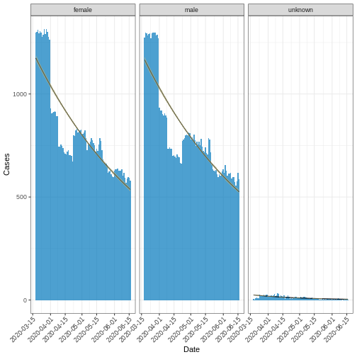
R
fitted_curve_poisson <-
  i2extras::fit_curve(
    x = df_incid,
    model = "poisson",
    alpha = 0.05
  )

base::plot(fitted_curve_poisson, angle = 45) +
  ggplot2::labs(x = "Date", y = "Cases")
Exponential growth or decay rate
The exponential growth or decay rate, denoted as \(r\), serves as an indicator for the trend in cases, indicating whether they are increasing (growth) or decreasing (decay) on an exponential scale. This rate is computed using the so-called renewal equation (Wallinga et al. 2006), which mechanistically links the reproductive number \(R\) of new cases to the generation interval of the disease. This computational method is implemented in the i2extras package.
Below is a code snippet demonstrating how to extract the growth/decay
rate from the above NB-fitted curve using the
growth_rate() function:
R
rates_nb <- i2extras::growth_rate(fitted_curve_nb)
rates_nb <- base::as.data.frame(rates_nb) |>
  subset(select = c(sex, r, r_lower, r_upper))
base::print(rates_nb)
OUTPUT
      sex            r      r_lower      r_upper
1  female -0.008241228 -0.009182635 -0.007300403
2    male -0.008346783 -0.009316775 -0.007377392
3 unknown -0.023703987 -0.028179436 -0.019299926Peak time
The Peak time is the time at which the highest
number of cases is observed in the aggregated data. It can be estimated
using the i2extras::estimate_peak() function as shown in
the below code chunk, which identify peak time from the
incidenc2 object df_incid.
R
peaks_nb <- i2extras::estimate_peak(df_incid, progress = FALSE) |>
  subset(select = -c(count_variable, bootstrap_peaks))

base::print(peaks_nb)
OUTPUT
# A data frame: 3 × 6
  sex     observed_peak observed_count lower_ci   median     upper_ci
* <chr>   <date>                 <int> <date>     <date>     <date>
1 female  2020-03-26              1314 2020-03-19 2020-03-23 2020-03-30
2 male    2020-03-27              1299 2020-03-18 2020-03-26 2020-03-30
3 unknown 2020-04-10                32 2020-03-24 2020-04-10 2020-04-16
Moving average
A moving or rolling average calculates the average number of cases
within a specified time period. This can be achieved by utilizing the
add_rolling_average() function from the
i2extras package on an incidence2 object.
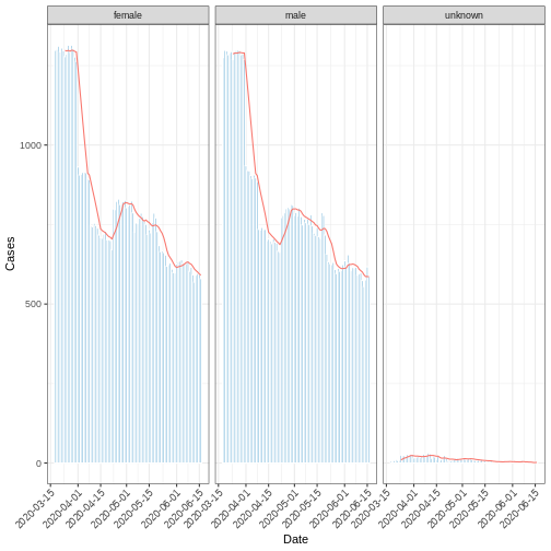
The following code chunk demonstrates the computation of the weekly
average number of cases from the incidence2 object
df_incid, followed by visualization.
R
library("ggplot2")

moving_Avg_week <- i2extras::add_rolling_average(df_incid, n = 7L)

base::plot(moving_Avg_week, border_colour = "white", angle = 45) +
  ggplot2::geom_line(
    ggplot2::aes(
      x = date_index,
      y = rolling_average,
      color = "red"
    )
  ) +
  ggplot2::labs(x = "Date", y = "Cases")
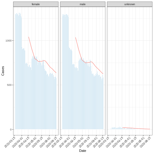
R
moving_Avg_mont <- i2extras::add_rolling_average(df_incid, n = 30L)

base::plot(
  moving_Avg_mont,
  border_colour = "white",
  angle = 45
) +
  ggplot2::geom_line(
    ggplot2::aes(
      x = date_index,
      y = rolling_average,
      color = "red"
    )
  ) +
  ggplot2::labs(x = "Date", y = "Cases")
Key Points
- Use i2extras to:
- fit epi-curve using either Poisson or
NB distributions,
- calculate exponential growth or decline of cases,
- find peak time, and
- computing moving average of cases in specified time window.
- fit epi-curve using either Poisson or
NB distributions,