Outbreak analytics pipelines
Last updated on 2024-11-04 | Edit this page
Estimated time: 12 minutes
Overview
Questions
- Why use R packages for Outbreak analytics?
- What can we do to analyse our outbreak data?
- How can I start doing Outbreak Analytics with R?
Objectives
- Explain our vision on the need for outbreak analytics R packages.
- Share our strategy to create R packages into an outbreak analytics pipeline.
- Define our plan to start your learning path in outbreak analytics with R.
Prerequisites
This episode requires you to be familiar with:
Data science : Basic programming with R.
Epidemic theory : Reproduction number.
Why to use R packages for Outbreak analytics?
Outbreaks appear with different diseases and in different contexts, but what all of them have in common are the key public health questions (Cori et al. 2017).
Is the epidemic going to take off? Is it under control? How much effort will be needed to control it? We can answer them by quantifying the transmissibility of the disease. The most used parameter for this is the reproduction number (\(R\)), the average number of secondary infections caused by a typical primary case in the population of interest (Prism, 2016). We can intuitively interpret it as:
- if \(R>1\), the epidemic is likely to grow,
- if \(R<1\), the epidemic is likely to decline.
We can estimate the reproduction number by initially using two data inputs: the incidence of reported cases and the generation time distribution. But to calculate it, we must apply the appropriate mathematical models written in code with the required computational methods. That is not enough! Following good practices, the code we write should be peer-reviewed and contain internal tests to double-check that we are getting the estimates we expect. Imagine rewriting all of it during a health emergency!
In R, the fundamental unit of shareable code is the package. A package bundles together code, data, documentation, and tests and is easy to share with others (Wickham and Bryan, 2023). We, as epidemiologists, can contribute to their collaborative maintenance as a community to perform less error-prone data analysis pipelines.
Questions to think about
Remember your last experience with outbreak data and reflect on these questions:
- What data sources did you need to understand the outbreak?
- How did you get access to that data?
- Is that analysis pipeline you followed reusable for the next response?
Reflect on your experiences.
Example: Quantify transmission
The EpiNow2 package provides a three-step solution to quantify the transmissibility. Let’s see how to do this with a minimal example. First, load the package:
R
library(EpiNow2)
First, get your case data
Case incidence data must be stored in a data frame with the observed number of cases per day. We can read an example from the package:
R
example_confirmed
OUTPUT
           date confirm
         <Date>   <num>
  1: 2020-02-22      14
  2: 2020-02-23      62
  3: 2020-02-24      53
  4: 2020-02-25      97
  5: 2020-02-26      93
 ---
126: 2020-06-26     296
127: 2020-06-27     255
128: 2020-06-28     175
129: 2020-06-29     174
130: 2020-06-30     126
Then, set the generation time
Not all primary cases have the same probability of generating a secondary case. The onset and cessation of infectiousness may occur gradually.
For EpiNow2, we can specify it as a probability
distribution adding its mean, standard
deviation (sd), and maximum value (max). To
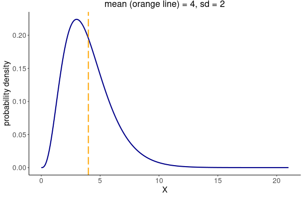
specify a generation time that follows a Gamma distribution
with mean \(\mu = 4\), standard
deviation \(\sigma^2 = 2\), and a
maximum value of 20, we write:
R
generation_time <- EpiNow2::Gamma(
  mean = 4,
  sd = 2,
  max = 20
)

generation_time
OUTPUT
- gamma distribution (max: 20):
  shape:
    4
  rate:
1As an example, we can show a generation time distribution from Manica et al., 2022
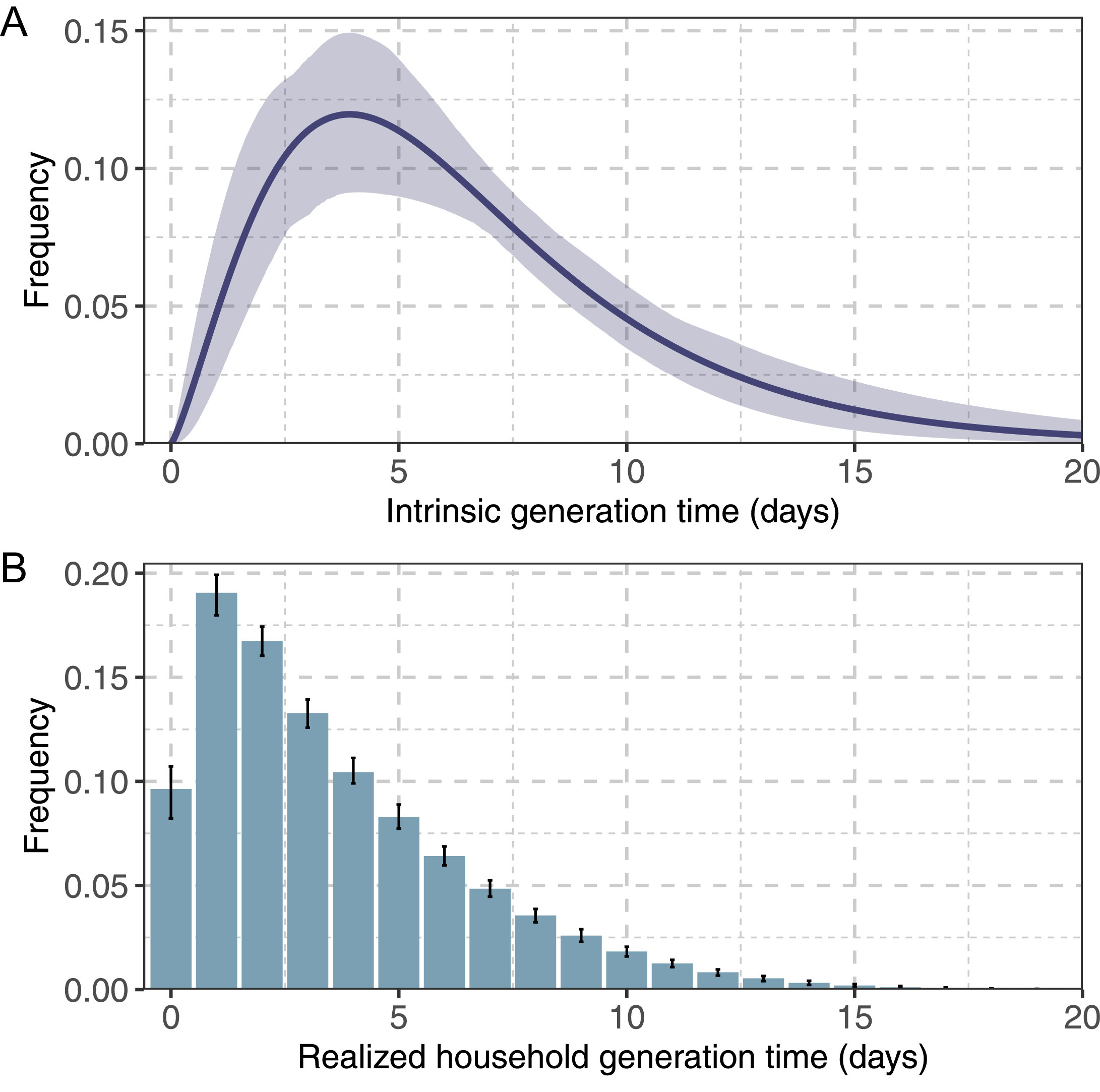
We can show the a figure from the Distribution Zoo.
A Gamma distribution with summary statistics of mean \(\mu = 4\) and standard deviation \(\sigma^2 = 2\), is equivalent to the distribution parameters of \(shape = 4\) and \(scale = 1\) (\(rate = 1/shape\)).
Now, let’s calculate the reproduction number!
In the epinow() function we can input these two
elements:
- the
reported_casesdata frame, and - the
generation_timedelay distribution, plus - the computation
stanparameters for this calculation:
R
epinow_estimates <- epinow(
  # cases
  data = example_confirmed[1:60],
  # delays
  generation_time = generation_time_opts(generation_time),
  # computation
  stan = stan_opts(cores = 4, samples = 1000)
)
OUTPUT
WARN [2024-11-04 18:53:49] epinow: Bulk Effective Samples Size (ESS) is too low, indicating posterior means and medians may be unreliable.
Running the chains for more iterations may help. See
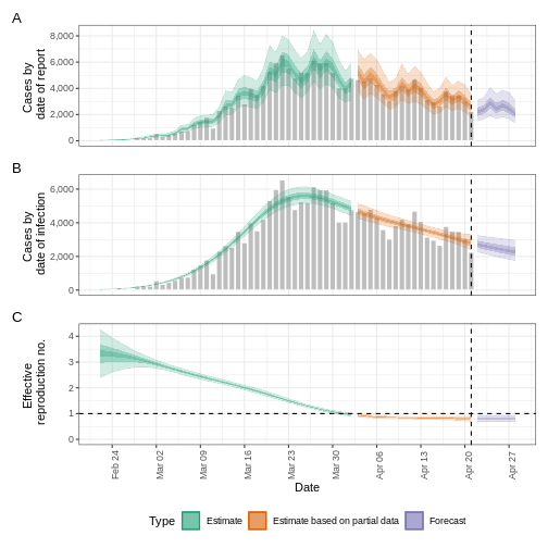
https://mc-stan.org/misc/warnings.html#bulk-ess - As an output, we get the time-varying (or effective) reproduction number, as well as the cases by date of report and date of infection:
R
base::plot(epinow_estimates)
Is this \(Rt\) estimation biased?
In the following episodes we are going to explore how to improve this initial estimate like adjusting by delays or incomplete observations.
In the meanwhile, we recommend you to review Gostic et al., 2020 on “Practical considerations for measuring the effective reproductive number, \(Rt\)” to avoid false precision in our reported \(Rt\) estimates.
The problem!
However, quantifying the transmissibility during a real-life outbreak response is more challenging than this example!
Usually, we receive outbreak data in non-standard formats, requiring specific steps and taking the most time to prepare usable data inputs. Some of them are:
- Read delay distributions from the literature
- Read and clean case data
- Validate your line list
- Describe case data
And this is not the end. After quantifying transmissibility we need to answer more key public health questions like: What is the attack rate we expect? What would be the impact of a given intervention? We can use the reproduction number and other outputs as new inputs for complementary tasks. For example:
- Estimate severity
- Create short-term forecast
- Simulate transmission scenarios
- Compare interventions
So, all these tasks can be interconnected in a pipeline:

What can we do?
Our strategy is gradually incorporating specialised R packages into our traditional analysis pipeline. These packages should fill the gaps in these epidemiology-specific tasks in response to outbreaks.
Epiverse-TRACE’s aim is to provide a software ecosystem for outbreak analytics. We support the development of software pieces, make the existing ones interoperable for the user experience, and stimulate a community of practice.
How can I start?
Our plan for these tutorials is to introduce key solutions from packages in all the tasks before and after the Quantify transmission task, plus the required theory concepts to interpret modelling outputs and make rigorous conclusions.
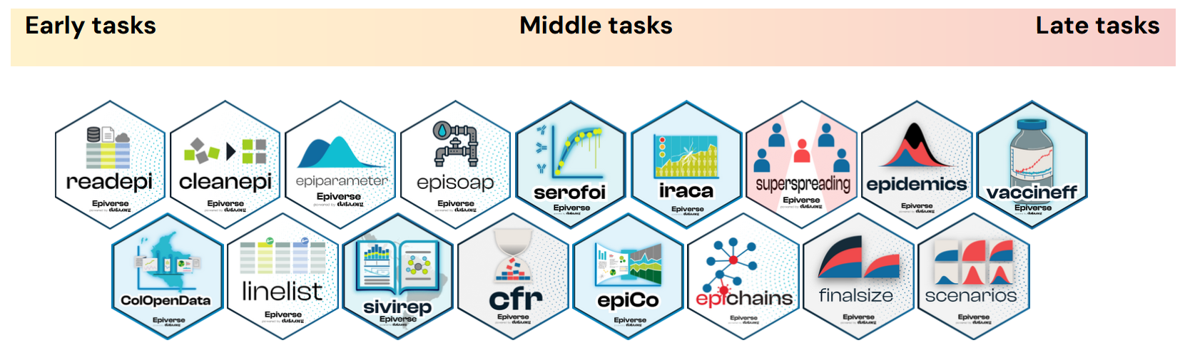
In the first set of episodes, you will learn how to optimise the reading of delay distributions and cleaning of case data to input them into the Quantify transmission task. These preliminary tasks are the Early tasks. These include packages like
{readepi}, cleanepi, linelist,{epiparameter}, and{episoap}.Then, we will get deeper into the packages and required theory to Quantify transmission and perform more real-time analysis tasks next to it. These are the Middle tasks. This includes EpiNow2, cfr, epichains, and
{superspreading}.Lastly, we will use Quantify transmission data outputs to compare it to other indicators and simulate epidemic scenarios as part of the Late tasks. This includes finalsize,
{epidemics}, and{scenarios}.
let’s start!
Lets start our learning path with the Early Task Tutorials!
Key Points
- Our vision is to have pipelines of R packages for outbreak analytics.
- Our strategy is to create interconnected tasks to get relevant outputs for public health questions.
- We plan to introduce package solutions and theory bits for each of the tasks in the outbreak analytics pipeline.