All in One View
Content from Introduction to outbreak analytics
Last updated on 2026-06-14 | Edit this page
Estimated time: 12 minutes
Overview
Questions
- How to calculate delays from line list data?
- Why it is important to account for delays in outbreak analytics?
Objectives
- Use the pipe operator
%>%to structure sequences of data operations. - Count observations in each group using
count()function. - Create new columns from existing columns using
mutate()function. - Keep or drop columns by their names using
select(). - Keep rows that match a condition using
filter(). - Create graphics declaratively using ggplot2.
Useful concepts maps to teach this episode are
Setup an RStudio project and folder
- Create an RStudio project. If needed, follow this how-to guide on “Hello RStudio Projects” to create one.
- Inside the RStudio project, create the
data/folder. - Inside the
data/folder, save the linelist.csv file.
RStudio projects
The directory of an RStudio Project named, for example
training, should look like this:
training/
|__ data/
|__ training.Rproj
RStudio Projects allows you to use relative
file paths with respect to the R Project, making your
code more portable and less error-prone. Avoids using
setwd() with absolute paths like
"C:/Users/MyName/WeirdPath/training/data/file.csv".
Challenge
Let’s starts by creating New Quarto Document!
- In the RStudio IDE, go to: File > New File > Quarto Document
- Accept the default options
- Save the file with the name
01-report.qmd - Use the
Renderbutton to render the file and preview the output.
Introduction
A new Ebola Virus Disease (EVD) outbreak has been notified in a country in West Africa. The Ministry of Health is coordinating the outbreak response and has contracted you as a consultant in epidemic analysis to inform the response in real-time. The available report of cases is coming from hospital admissions.
Let’s start by loading the package readr to read
.csv data, dplyr to manipulate data,
tidyr to rearrange it, and here to write
file paths within your RStudio project. We’ll use the pipe
%>% to connect some of their functions, including others
from the package ggplot2, so let’s call to the package
tidyverse that loads them all:
R
# Load packages
library(tidyverse) # loads readr, dplyr, tidyr and ggplot2
OUTPUT
── Attaching core tidyverse packages ──────────────────────── tidyverse 2.0.0 ──
✔ dplyr     1.2.1     ✔ readr     2.2.0
✔ forcats   1.0.1     ✔ stringr   1.6.0
✔ ggplot2   4.0.3     ✔ tibble    3.3.1
✔ lubridate 1.9.5     ✔ tidyr     1.3.2
✔ purrr     1.2.2
── Conflicts ────────────────────────────────────────── tidyverse_conflicts() ──
✖ dplyr::filter() masks stats::filter()
✖ dplyr::lag()    masks stats::lag()
ℹ Use the conflicted package (<http://conflicted.r-lib.org/>) to force all conflicts to become errorsThe double-colon
The double-colon :: in R let you call a specific
function from a package without loading the entire package into the
current environment.
For example, dplyr::filter(data, condition) uses
filter() from the dplyr package.
This helps us remember package functions and avoid namespace conflicts.
Explore data
For the purpose of this episode, we will read a pre-cleaned line list data. Following episodes will tackle how to solve cleaning tasks.
R
# Read data
# e.g.: if path to file is data/linelist.csv then:
cases <- readr::read_csv(
  here::here("data", "linelist.csv")
)
Why should we use the {here} package?
The package here simplifies file referencing in R projects. It allows them to work across different operating systems (Windows, Mac, Linux). This feature, called cross-environment compatibility, eliminates the need to adjust file paths. For example:
- On Windows, paths are written using backslashes (
\) as the separator between folder names:"data\raw-data\file.csv" - On Unix based operating system such as macOS or Linux the forward
slash (
/) is used as the path separator:"data/raw-data/file.csv"
The here package adds one more layer of reproducibility to your work. For more, read this tutorial about open, sustainable, and reproducible epidemic analysis with R
R
# Print line list data
cases
OUTPUT
# A tibble: 166 × 11
   case_id generation date_of_infection date_of_onset date_of_hospitalisation
   <chr>        <dbl> <date>            <date>        <date>
 1 d1fafd           0 NA                2014-04-07    2014-04-17
 2 53371b           1 2014-04-09        2014-04-15    2014-04-20
 3 f5c3d8           1 2014-04-18        2014-04-21    2014-04-25
 4 e66fa4           2 NA                2014-04-21    2014-05-06
 5 49731d           0 2014-03-19        2014-04-25    2014-05-02
 6 0f58c4           2 2014-04-22        2014-04-26    2014-04-29
 7 6c286a           2 NA                2014-04-27    2014-04-27
 8 881bd4           3 2014-04-26        2014-05-01    2014-05-05
 9 d58402           2 2014-04-23        2014-05-01    2014-05-10
10 f9149b           3 NA                2014-05-03    2014-05-04
# ℹ 156 more rows
# ℹ 6 more variables: date_of_outcome <date>, outcome <chr>, gender <chr>,
# hospital <chr>, lon <dbl>, lat <dbl>Take a moment to review the data and its structure..
- Do the data and format resemble line lists you’ve encountered before?
- If you were part of the outbreak investigation team, what additional information might you want to collect?
The information to collect will depend on the questions we need to give a response.
At the beginning of an outbreak, we need data to give a response to questions like:
- How fast does an epidemic grow?
- What is the risk of death?
- How many cases can I expect in the coming days?
Informative indicators are:
- growth rate, reproduction number.
- case fatality risk, hospitalization fatality risk.
- projection or forecast of cases.
Useful data are:
- date of onset, date of death.
- delays from infection to onset, from onset to death.
- percentage of observations detected by surveillance system.
- subject characteristics to stratify the analysis by person, place, time.
You may notice that there are missing entries.
We can also explore missing data with summary a visualization:
R
cases %>%
  visdat::vis_miss()
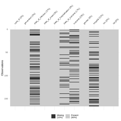
Why do we have more missings on date of infection or date of outcome?
- date of infection: mostly unknown, depended on limited coverage of contact tracing or outbreak research, and sensitive to recall bias from subjects.
- date of outcome: reporting delay
Calculate severity
A frequent indicator for measuring severity is the Case Fatality Risk (CFR).
CFR is defined as the conditional probability of death given confirmed diagnosis, calculated as the cumulative number of deaths from an infectious disease over the number of confirmed diagnosed cases.
We can use the function dplyr::count() to count the
observations in each group of the variable outcome:
R
cases %>%
  dplyr::count(outcome)
OUTPUT
# A tibble: 3 × 2
  outcome     n
  <chr>   <int>
1 Death      65
2 Recover    59
3 <NA> 42Report:
What to do with cases whose outcome is
<NA>?Should we consider missing outcomes to calculate the CFR?
Keeping cases with missing outcome is useful to track the incidence of number of new cases, useful to assess transmission.
However, when assessing severity, CFR estimation is sensitive to:
Right-censoring bias. If we include observations with unknown final status we can underestimate the true CFR.
Selection bias. At the beginning of an outbreak, given that health systems collect most clinically severe cases, an early estimate of the CFR can overestimate the true CFR.
Data of today will not include outcomes from patients that are still hospitalised. Then, one relevant question to ask is: In average, how much time it would take to know the outcomes of hospitalised cases? For this we can calculate delays!
Calculate delays
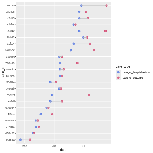
The time between sequence of dated events can vary between subjects. For example, we would expect the date of infection to always be before the date of symptom onset, and the later always before the date of hospitalization.
In a random sample of 30 observations from the cases
data frame we observe variability between the date of hospitalization
and date of outcome:
We can calculate the average time from hospitalisation to outcome from the line list.
From the cases object we will use:
-
dplyr::select()to keep columns using their names, -
dplyr::mutate()to create one new columnoutcome_delayas a function of existing variablesdate_of_outcomeanddate_of_hospitalisation, -
dplyr::filter()to keep the rows that match a condition likeoutcome_delay > 0, -
skimr::skim()to get useful summary statistics
R
# delay from report to outcome
cases %>%
  dplyr::select(case_id, date_of_hospitalisation, date_of_outcome) %>%
  dplyr::mutate(outcome_delay = date_of_outcome - date_of_hospitalisation) %>%
  dplyr::filter(outcome_delay > 0) %>%
  skimr::skim(outcome_delay)
| Name | Piped data |
| Number of rows | 123 |
| Number of columns | 4 |
| _______________________ | |
| Column type frequency: | |
| difftime | 1 |
| ________________________ | |
| Group variables | None |
Variable type: difftime
| skim_variable | n_missing | complete_rate | min | max | median | n_unique |
|---|---|---|---|---|---|---|
| outcome_delay | 0 | 1 | 1 days | 55 days | 7 days | 29 |
Inconsistencies among sequence of dated-events?
Wait! Is it consistent to have negative time delays from primary to secondary observations, i.e., from hospitalisation to death?
In the next episode called Clean data we will learn how to check sequence of dated-events and other frequent and challenging inconsistencies!
Challenge
To calculate a delay-adjusted Case Fatality Risk (CFR), we need to assume a known delay from onset to death.
Using the cases object:
- Calculate the summary statistics of the delay from onset to death.
Keep the rows that match a condition like
outcome == "Death":
R
# delay from onset to death
cases %>%
  dplyr::filter(outcome == "Death") %>%
  ...() # replace ... with downstream code
Is it consistent to have negative delays from onset of symptoms to death?
R
# delay from onset to death
cases %>%
  dplyr::select(case_id, date_of_onset, date_of_outcome, outcome) %>%
  dplyr::filter(outcome == "Death") %>%
  dplyr::mutate(delay_onset_death = date_of_outcome - date_of_onset) %>%
  dplyr::filter(delay_onset_death > 0) %>%
  skimr::skim(delay_onset_death)
| Name | Piped data |
| Number of rows | 46 |
| Number of columns | 5 |
| _______________________ | |
| Column type frequency: | |
| difftime | 1 |
| ________________________ | |
| Group variables | None |
Variable type: difftime
| skim_variable | n_missing | complete_rate | min | max | median | n_unique |
|---|---|---|---|---|---|---|
| delay_onset_death | 0 | 1 | 2 days | 17 days | 7 days | 15 |
Where is the source of the inconsistency? Let’s say you want to keep the rows with negative delay values to investigate them. How would you do it?
We can use dplyr::filter() again to identify the
inconsistent observations:
R
# keep negative delays
cases %>%
  dplyr::select(case_id, date_of_onset, date_of_outcome, outcome) %>%
  dplyr::filter(outcome == "Death") %>%
  dplyr::mutate(delay_onset_death = date_of_outcome - date_of_onset) %>%
  dplyr::filter(delay_onset_death < 0)
OUTPUT
# A tibble: 6 × 5
  case_id date_of_onset date_of_outcome outcome delay_onset_death
  <chr>   <date>        <date>          <chr>   <drtn>
1 c43190  2014-05-06    2014-04-26      Death   -10 days
2 bd8c0e  2014-05-17    2014-05-09      Death    -8 days
3 49d786  2014-05-20    2014-05-11      Death    -9 days
4 e85785  2014-06-03    2014-06-02      Death    -1 days
5 60f0c2  2014-06-07    2014-05-30      Death    -8 days
6 a48f5d  2014-06-15    2014-06-10      Death    -5 days
More on estimating a delay-adjusted Case Fatality Risk (CFR) on the episode about Estimating outbreak severity!
Epidemic curve
The first question we want to know is simply: how bad is it? The first step of the analysis is descriptive. We want to draw an epidemic curve or epicurve. This visualises the incidence over time by date of symptom onset.
From the cases object we will use:
-
ggplot()to declare the input data frame, -
aes()for the variabledate_of_onsetto map togeoms, -
geom_histogram()to visualise the distribution of a single continuous variable with abinwidthequal to 7 days.
R
# incidence curve
cases %>%
  ggplot(aes(x = date_of_onset)) +
  geom_histogram(binwidth = 7)
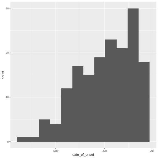
The early phase of an outbreak usually growths exponentially.
- Why exponential growth may not be observed in the most recent weeks?
Close inspection of the line list shows that the last date of any entry (by date of hospitalization) is a bit later than the last date of symptom onset.
From the cases object we can use:
-
dplyr::summarise()to summarise each group down to one row, -
base::maxto calculate the maximum dates of onset and hospitalisation.
When showcasing this to learners in a live coding session, you can
also use cases %>% view() to rearrange by date
columns.
R
cases %>%
  dplyr::summarise(
    max_onset = max(date_of_onset),
    max_hospital = max(date_of_hospitalisation)
  )
OUTPUT
# A tibble: 1 × 2
  max_onset  max_hospital
  <date>     <date>
1 2014-06-27 2014-07-07
You may want to examine how long after onset of symptoms cases are hospitalised; this may inform the reporting delay from this line list data:
R
# reporting delay
cases %>%
  dplyr::select(case_id, date_of_onset, date_of_hospitalisation) %>%
  dplyr::mutate(reporting_delay = date_of_hospitalisation - date_of_onset) %>%
  ggplot(aes(x = reporting_delay)) +
  geom_histogram(binwidth = 1)
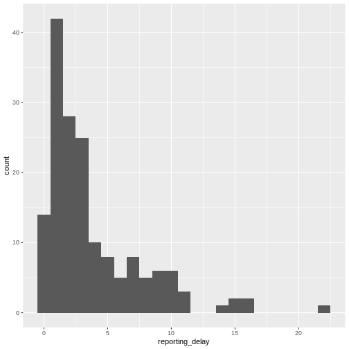
The distribution of the reporting delay in day units is heavily skewed. Symptomatic cases may take up to two weeks to be reported.
From reports (hospitalisations) in the most recent two weeks, we completed the exponential growth trend of incidence cases within the last four weeks:
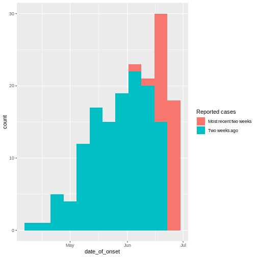
Given to reporting delays during this outbreak, it seemed that two weeks ago we had a decay of cases during the last three weeks. We needed to wait a couple of weeks to complete the incidence of cases on each week.
Challenge
Report:
- What indicator can we use to estimate transmission from the incidence curve?
- The growth rate! by fitting a linear model.
- The reproduction number accounting for delays from secondary observations to infection.
More on this topic on episodes about Aggregate and visualize and Quantifying transmission.
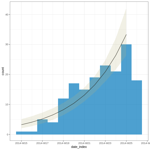
OUTPUT
# A tibble: 2 × 6
  count_variable term        estimate std.error statistic  p.value
  <chr>          <chr>          <dbl>     <dbl>     <dbl>    <dbl>
1 date_of_onset  (Intercept) -537.      70.1        -7.67 1.76e-14
2 date_of_onset  date_index     0.233    0.0302      7.71 1.29e-14
Note: Due to the diagnosed reporting delay, We conveniently truncated the epidemic curve one week before to fit the model! This improves the fitted model to data when quantifying the growth rate during the exponential phase.
In order to account for these epidemiological delays when estimating indicators of severity or transmission, in our analysis we need to input delays as Probability Distributions. We will learn how to fit and access them in the next episodes.
Challenges
Challenge
Relevant delays when estimating transmission
Review the definition of the incubation period in our glossary page.
Calculate the summary statistics of the incubation period distribution observed in the line list.
Visualize the distribution of the incubation period from the line list.
Calculate the summary statistics:
R
cases %>%
  dplyr::select(case_id, date_of_infection, date_of_onset) %>%
  dplyr::mutate(incubation_period = date_of_onset - date_of_infection) %>%
  skimr::skim(incubation_period)
| Name | Piped data |
| Number of rows | 166 |
| Number of columns | 4 |
| _______________________ | |
| Column type frequency: | |
| difftime | 1 |
| ________________________ | |
| Group variables | None |
Variable type: difftime
| skim_variable | n_missing | complete_rate | min | max | median | n_unique |
|---|---|---|---|---|---|---|
| incubation_period | 61 | 0.63 | 1 days | 37 days | 5 days | 25 |
Visualize the distribution:
R
cases %>%
  dplyr::select(case_id, date_of_infection, date_of_onset) %>%
  dplyr::mutate(incubation_period = date_of_onset - date_of_infection) %>%
  ggplot(aes(x = incubation_period)) +
  geom_histogram(binwidth = 1)

In coming episode we will learn how to fit statistical distribution paramaters to a distribution, or access to the most appropriate estimates.
With the distribution parameters of the incubation period we can infer the length of active monitoring or quarantine. Lauer et al., 2020 estimated the incubation period of Coronavirus Disease 2019 (COVID-19) from publicly reported confirmed cases.
References
Cori, A. et al. (2019) Real-time outbreak analysis: Ebola as a case study - part 1 · Recon Learn, RECON learn. Available at: https://www.reconlearn.org/post/real-time-response-1 (Accessed: 06 November 2024).
Cori, A. et al. (2019) Real-time outbreak analysis: Ebola as a case study - part 2 · Recon Learn, RECON learn. Available at: https://www.reconlearn.org/post/real-time-response-2 (Accessed: 07 November 2024).
Content from Introduction to delays
Last updated on 2026-06-14 | Edit this page
Estimated time: 12 minutes
Overview
Questions
- How to fit a probability distribution to delay data?
- How to interpret distribution parameters?
- How to access distribution parameters from fitting objects
Objectives
- Fit a probability distribution to data using fitdistrplus
- Extract a single column using
pull(), dollar sign$, or square brackets[].
Introduction
Delays are key for downstream task in outbreak analytics. To estimate the outbreak severity, we need to assume a known delay from onset to death. To quantify transmission, we need to consider delays from the moment of infection to the time of data collection. In order to account for epidemiological delays when estimating indicators of severity or transmission, in our analysis we need to input delays as Probability Distributions.
Let’s start by loading the package dplyr to manipulate
data. We’ll use the pipe %>% to connect some of their
functions, including others from the package ggplot2, so
let’s call to the package tidyverse that loads them all.
We will also use fitdistrplus to fit probability
distributions to delays:
R
# Load packages
library(tidyverse) # loads dplyr, the pipe, and ggplot2
library(fitdistrplus)
The double-colon
The double-colon :: in R let you call a specific
function from a package without loading the entire package into the
current environment.
For example, dplyr::filter(data, condition) uses
filter() from the dplyr package.
This helps us remember package functions and avoid namespace conflicts.
Fit a probability distribution to delays
Assess learners based on video refreshers on distributions, likelihood, and maximum likelihood from setup instructions.
We fit a probability distribution to data (like delays) to make inferences about it. These inferences can be useful for Public health interventions and decision making. For example:
From the incubation period distribution we can inform the length of active monitoring or quarantine. We can infer the time by which 99% of infected individuals are expected to show symptoms (Lauer et al., 2020).
From the serial interval distribution we can optimize contact tracing. We can evaluate the need to expand the number of days pre-onset to consider in the contact tracing to include more backwards contacts (Claire Blackmore, 2021; Davis et al., 2020).
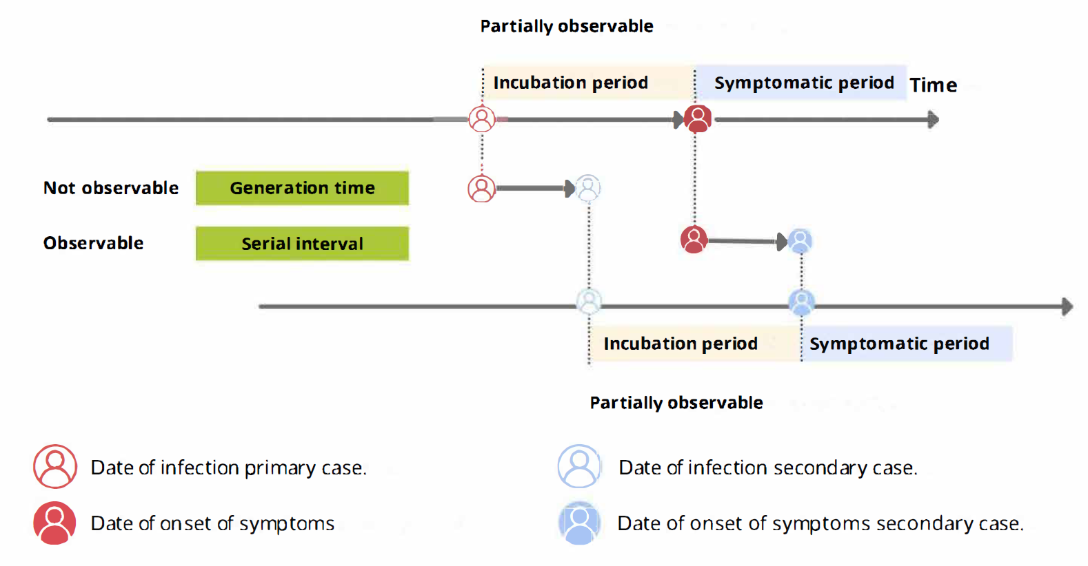
From time periods to probability distributions
When we calculate the serial interval, we see that not all case pairs have the same time length. We will observe this variability for any case pair and individual time period.
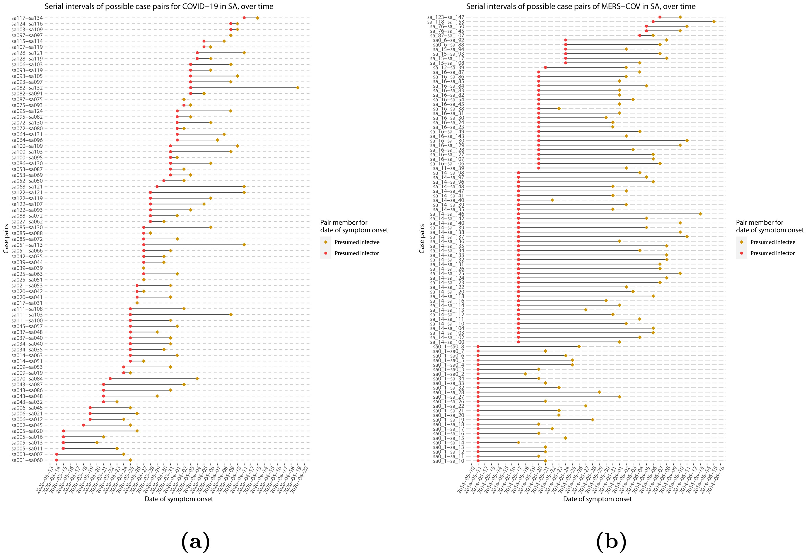
To summarise these data from individual and pair time periods, we can find the statistical distributions that best fit the data (McFarland et al., 2023).
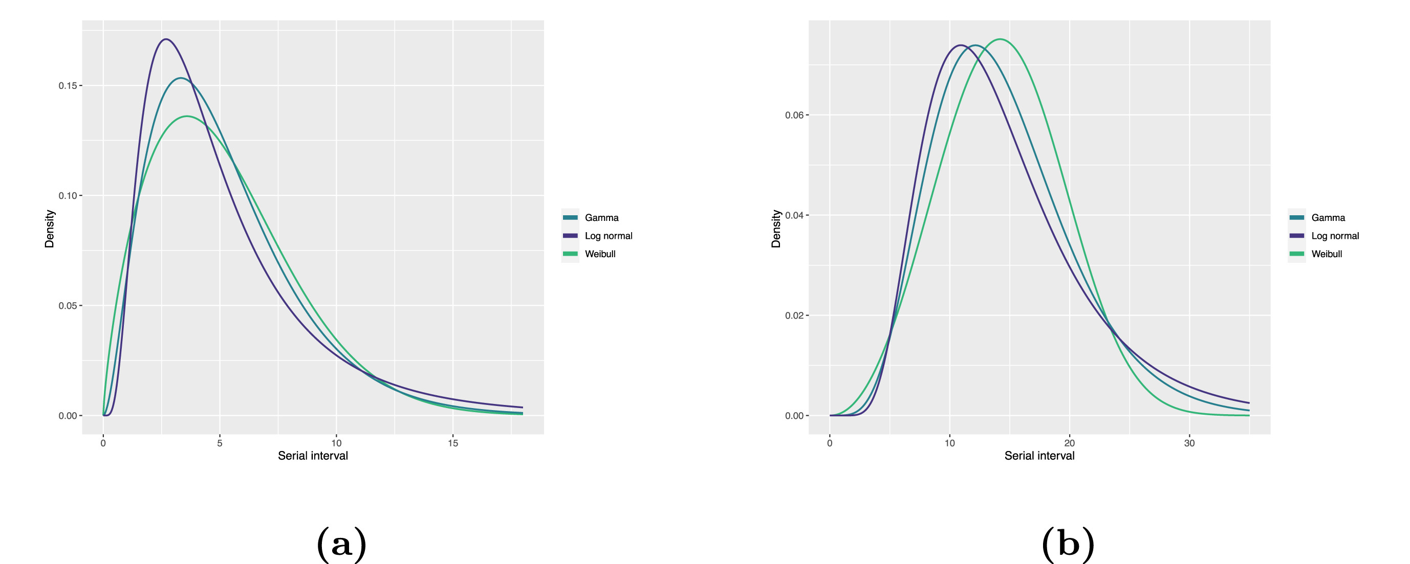
Statistical distributions are summarised in terms of their summary statistics like the location (mean and percentiles) and spread (variance or standard deviation) of the distribution, or with their distribution parameters that inform about the form (shape and rate/scale) of the distribution. These estimated values can be reported with their uncertainty (95% confidence intervals).
| Gamma | mean | shape | rate/scale |
|---|---|---|---|
| MERS-CoV | 14.13(13.9–14.7) | 6.31(4.88–8.52) | 0.43(0.33–0.60) |
| COVID-19 | 5.1(5.0–5.5) | 2.77(2.09–3.88) | 0.53(0.38–0.76) |
| Weibull | mean | shape | rate/scale |
|---|---|---|---|
| MERS-CoV | 14.2(13.3–15.2) | 3.07(2.64–3.63) | 16.1(15.0–17.1) |
| COVID-19 | 5.2(4.6–5.9) | 1.74(1.46–2.11) | 5.83(5.08–6.67) |
| Log normal | mean | mean-log | sd-log |
|---|---|---|---|
| MERS-CoV | 14.08(13.1–15.2) | 2.58(2.50–2.68) | 0.44(0.39–0.5) |
| COVID-19 | 5.2(4.2–6.5) | 1.45(1.31–1.61) | 0.63(0.54–0.74) |
To illustrate this, let’s continue with the same line list from the previous episode:
R
# Read data
# e.g.: if path to file is data/linelist.csv then:
cases <- readr::read_csv(
  here::here("data", "linelist.csv")
)
From the cases object we can use:
-
dplyr::mutate()to transform thereporting_delayclass object from<time>to<numeric>, -
dplyr::filter()to keep the positive values, -
dplyr::pull()to extract a single column, -
fitdistrplus::fitdist()to fit a probability distribution using Maximum Likelihood. We can test distributions like the Log Normal ("lnorm"),"gamma", or"weibull".
R
cases %>%
dplyr::select(case_id, date_of_onset, date_of_hospitalisation) %>%
dplyr::mutate(reporting_delay = date_of_hospitalisation - date_of_onset) %>%
dplyr::mutate(reporting_delay_num = as.numeric(reporting_delay)) %>%
dplyr::filter(reporting_delay_num > 0) %>%
dplyr::pull(reporting_delay_num) %>%
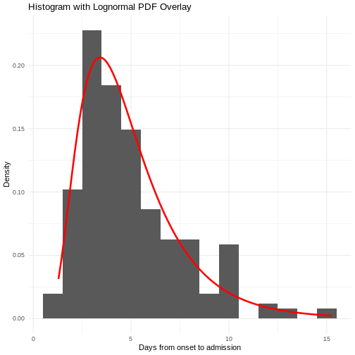
fitdistrplus::fitdist(distr = "lnorm")
OUTPUT
Fitting of the distribution ' lnorm ' by maximum likelihood
Parameters:
         estimate Std. Error
meanlog 1.0488098 0.06866105
sdlog   0.8465102 0.04855039
Use summary() to find goodness-of-fit statistics from
the Maximum likelihood. Use plot() to visualize the fitted
density function and other quality control plots. To compare multiple
distributions you can use superspreading::ic_tbl().
We’ll explore that package later!
Now we can do inferences from the probability distribution fitted to the epidemiological delay! Want to learn how? Read the “Show details” :)
Making inferences from probability distributions
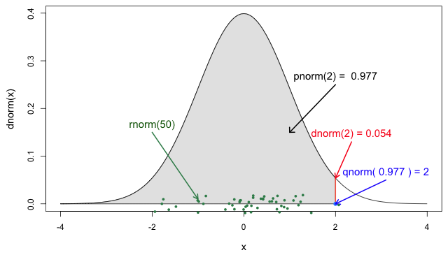
From probability distributions we can infer estimates like cumulative probability, maximum values, or generate random values. We can access to them using R probability functions.
We recommend you read the definitions of the R probability functions for the Normal distribution. From it we can relate with any other family of statistical distributions!
Each probability distribution has a unique set of
parameters and probability functions.
Read the Distributions
in the stats package or ?stats::Distributions to find
the ones available in R.
For example, assuming that the reporting delay follows a Log
Normal distribution, we can use plnorm() to
calculate the probability of observing a reporting delay of 14 days or
less:
R
plnorm(q = 14, meanlog = 1.0488098, sdlog = 0.8465102)
OUTPUT
[1] 0.9698499Or the amount of time by which 99% of symptomatic individuals are expected to be reported in the hospitalization record:
R
qlnorm(p = 0.99, meanlog = 1.0488098, sdlog = 0.8465102)
OUTPUT
[1] 20.45213You will find more examples of how to use delays for decision-making at the Use delay distributions in analysis at Tutorials Middle!
To interactively explore probability distributions, their parameters and access to their distribution functions, we suggest to explore a shinyapp called The Distribution Zoo: https://ben18785.shinyapps.io/distribution-zoo/
Let’s review some operators used until now:
- Assignment
<-assigns a value to a variable from right to left. - Double colon
::to call a function from a specific package. - Pipe
%>%to structure sequences of data operations left-to-right
We need to add two more to the list:
- Dollar sign
$ - Square brackets
[]
Last step is to access to this parameters. Most modeling outputs from
R functions will be stored as list class objects. In R, the
dollar sign operator $ is used to access elements (like
columns) within a data frame or list by name, allowing for easy
retrieval of specific components.
A code completion tip
If we write the square brackets [] next
to the object reporting_delay_fit$estimate[], within
[] we can use the Tab key ↹ for code
completion feature
This gives quick access to "meanlog" and
"sdlog". We invite you to try this out in code chunks and
the R console!
R
# 1. Place the cursor within the square brackets
# 2. Use the Tab key
# 3. Explore the completion list
# 4. Select for "meanlog" or "sdlog"
reporting_delay_fit$estimate[]
Estimating epidemiological delays is CHALLENGING!
Epidemiological delays need to account for biases like censoring, right truncation, or epidemic phase (Charniga et al., 2024).
Additionally, at the beginning of an outbreak, limited data or resources exist to perform this during a real-time analysis. Until we have more appropriate data for the specific disease and region of the ongoing outbreak, we can reuse delays from past outbreaks from the same pathogens or close in its phylogeny, independent of the area of origin.
Next step
In the following tutorial episodes, we will:
- Efficiently clean and produce epidemic curves to explore patterns of disease spread by different groups and time aggregates. Find more in Tutorials Early!
- Access to epidemiological delay distributions to estimate delay-adjusted transmission and severity metrics (e.g. reproduction number and case fatality risk). Find more in Tutorials Middle!
- Use parameter values like the basic reproduction number, and delays like the latent period and infectious period to simulate transmission trajectories and intervention scenarios. Find more in Tutorials Late!
Challenges
Challenge
Relevant delays when estimating transmission
Review the definition of the incubation period in our glossary page.
Calculate the summary statistics of the incubation period distribution observed in the line list.
Visualize the distribution of the incubation period from the line list.
Fit a log-normal distribution to get the probability distribution parameters of the the observed incubation period.
(Optional) Infer the time by which 99% of infected individuals are expected to show symptoms.
Calculate the summary statistics:
R
cases %>%
  dplyr::select(case_id, date_of_infection, date_of_onset) %>%
  dplyr::mutate(incubation_period = date_of_onset - date_of_infection) %>%
  skimr::skim(incubation_period)
| Name | Piped data |
| Number of rows | 166 |
| Number of columns | 4 |
| _______________________ | |
| Column type frequency: | |
| difftime | 1 |
| ________________________ | |
| Group variables | None |
Variable type: difftime
| skim_variable | n_missing | complete_rate | min | max | median | n_unique |
|---|---|---|---|---|---|---|
| incubation_period | 61 | 0.63 | 1 days | 37 days | 5 days | 25 |
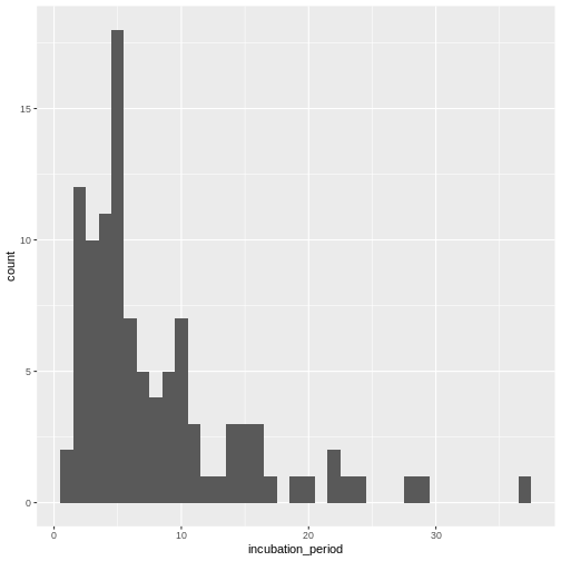
Visualize the distribution:
R
cases %>%
  dplyr::select(case_id, date_of_infection, date_of_onset) %>%
  dplyr::mutate(incubation_period = date_of_onset - date_of_infection) %>%
  ggplot(aes(x = incubation_period)) +
  geom_histogram(binwidth = 1)
Fit a log-normal distribution:
R
incubation_period_dist <- cases %>%
  dplyr::select(case_id, date_of_infection, date_of_onset) %>%
  dplyr::mutate(incubation_period = date_of_onset - date_of_infection) %>%
  mutate(incubation_period_num = as.numeric(incubation_period)) %>%
  filter(!is.na(incubation_period_num)) %>%
  pull(incubation_period_num) %>%
  fitdistrplus::fitdist(distr = "lnorm")

incubation_period_dist
OUTPUT
Fitting of the distribution ' lnorm ' by maximum likelihood
Parameters:
         estimate Std. Error
meanlog 1.8037993 0.07381350
sdlog   0.7563633 0.05219361
(Optional) Infer the time by which 99% of infected individuals are expected to show symptoms:
R
qlnorm(
  p = 0.99,
  meanlog = incubation_period_dist$estimate["meanlog"],
  sdlog = incubation_period_dist$estimate["sdlog"]
)
OUTPUT
[1] 35.28167With the distribution parameters of the incubation period we can infer the length of active monitoring or quarantine. Lauer et al., 2020 estimated the incubation period of Coronavirus Disease 2019 (COVID-19) from publicly reported confirmed cases.
- Epidemiological delays condition the estimation of indicators for severity or transmission.
- Fit probability distribution to delays to make inferences from them for decision-making.
- Fitting epidemiological delays need to account for biases like censoring, right truncation, or epidemic phase.
References
Cori, A. et al. (2019) Real-time outbreak analysis: Ebola as a case study - part 1 · Recon Learn, RECON learn. Available at: https://www.reconlearn.org/post/real-time-response-1 (Accessed: 06 November 2024).
Cori, A. et al. (2019) Real-time outbreak analysis: Ebola as a case study - part 2 · Recon Learn, RECON learn. Available at: https://www.reconlearn.org/post/real-time-response-2 (Accessed: 07 November 2024).