Estimating the proportion of cases that are ascertained during an outbreak • cfr

The ascertainment of cases during an outbreak is influenced by a multiple factor including testing capacity, the case definition, and sampling regime (e.g. symptom-based testing rather than random sampling). estimate_ascertainment() offers a convenient way to calculate the proportion of cases that is ascertained using a cases and deaths time-series, a baseline “known” severity, and optionally a distribution of delays between case reporting and death.

The ascertainment ratio is calculated as the disease severity calculated from the data, divided by the “known” disease severity known or assumed from our best knowledge of the pathology of the disease.

estimate_ascertainment() uses cfr_static() internally to estimate the delay-adjusted severity of the disease.

New to calculating disease severity using cfr? You might want to see the “Get started” vignette first.

Use case

The ascertainment of cases in an outbreak is not perfect. We want to estimate the proportion of cases being ascertained given case and death data.

What we have

A time-series of cases and deaths, (cases may be substituted by another indicator of infections over time);
Data on the distribution of delays, describing the probability an individual will die \(t\) days after they were initially infected.

Code

# load {cfr} and data packages
library(cfr)

# packages to wrangle and plot data
library(dplyr)
library(tidyr)
library(purrr)
library(scales)
library(forcats)
library(ggplot2)

Ascertainment for the Covid-19 pandemic in the U.K.

This example shows ascertainment ratio estimation using cfr and data from the Covid-19 pandemic in the United Kingdom.

We load example Covid-19 daily case and death data provided with the cfr package as covid_data, and subset for the first six months of U.K. data.

Code

# get Covid data provided with the package
data("covid_data")

# filter for the U.K
df_covid_uk <- filter(
  covid_data,
  country == "United Kingdom", date <= "2020-06-30"
)

# view the data format
tail(df_covid_uk)
#>           date        country cases deaths
#> 175 2020-06-25 United Kingdom   883     97
#> 176 2020-06-26 United Kingdom   777    101
#> 177 2020-06-27 United Kingdom   726    108
#> 178 2020-06-28 United Kingdom   666     79
#> 179 2020-06-29 United Kingdom   653     73
#> 180 2020-06-30 United Kingdom   449     70

We obtain the appropriate distribution reported in Linton et al. (2020); this is a log-normal distribution with \(\mu\) = 2.577 and \(\sigma\) = 0.440.

Note that Linton et al. (2020) fitted a discrete lognormal distribution — but we use a continuous distribution here. See the vignette on delay distributions for more on when using a continuous instead of discrete distribution is acceptable, and on using discrete distributions with cfr.

Note that we use the central estimates for each distribution parameter, and by ignoring uncertainty in these parameters the uncertainty in the resulting CFR is likely to be underestimated.

Estimating the proportion of cases that have been ascertained

We use the estimate_ascertainment() function to calculate the static CFR (internally), and the overall ascertainment for the Covid-19 pandemic in the U.K.

We assume that the “true” CFR of Covid-19 is 0.014 (i.e. 1.4%) (Verity et al. 2020). Future plans for this package include ability to incorporate uncertainty in CFR estimates when calculating under-ascertainment.

Note that the CFR from Verity et al. (2020) is based on lab-confirmed and clinically diagnosed cases from Wuhan, China. Since the case definition for the U.K. is different from that used here, the ascertainment ratio estimated is likely to be biased.

Furthermore, by ignoring uncertainty in this estimate, the ascertainment ratio is likely to be over-precise as well.

Code

# static ascertainment on data
estimate_ascertainment(
  data = df_covid_uk,
  delay_density = function(x) dlnorm(x, meanlog = 2.577, sdlog = 0.440),
  severity_baseline = 0.014
)
#> Total cases = 283420 and p = 0.206: using Normal approximation to binomial likelihood.
#>   ascertainment_mean ascertainment_low ascertainment_high
#> 1         0.09810792        0.02316347          0.2167183

Ascertainment in countries with large early Covid-19 pandemics

Finally, we estimate ascertainment for all countries with at least 100,000 reported Covid-19 deaths between 2020 and 2023, and focus on the period between the start of each outbreak to the 1st of June 2020.

We now use the larger dataset covid_data made available with the cfr package. We exclude four countries which only provide weekly data (with zeros for dates in between), and plot the ascertainment for each country remaining.

Code

# countries with weekly reporting
weekly_reporting <- c("France", "Germany", "Spain", "Ukraine")

# subset for early covid outbreaks
covid_data_early <- filter(
  covid_data, date < "2020-06-01",
  !country %in% weekly_reporting
)

# nest the data
df_reporting <- nest(covid_data_early, .by = country)

# define density function
delay_density <- function(x) dlnorm(x, meanlog = 2.577, sdlog = 0.440)

# calculate the reporting rate in each country using
# map on nested dataframes
df_reporting <- mutate(
  df_reporting,
  reporting = map(
    .x = data, .f = estimate_ascertainment,
    # arguments to function
    severity_baseline = 0.014,
    delay_density = delay_density
  )
)
#> Total cases = 22406 and p = 0.108: using Normal approximation to binomial likelihood.
#> Total cases = 465166 and p = 0.125: using Normal approximation to binomial likelihood.
#> Total cases = 26778 and p = 0.0593: using Normal approximation to binomial likelihood.
#> Total cases = 182148 and p = 0.0553: using Normal approximation to binomial likelihood.
#> Total cases = 26477 and p = 0.0913: using Normal approximation to binomial likelihood.
#> Total cases = 148950 and p = 0.0652: using Normal approximation to binomial likelihood.
#> Total cases = 232664 and p = 0.149: using Normal approximation to binomial likelihood.
#> Total cases = 120229 and p = 0.286: using Normal approximation to binomial likelihood.
#> Total cases = 148285 and p = 0.231: using Normal approximation to binomial likelihood.
#> Total cases = 23571 and p = 0.0585: using Normal approximation to binomial likelihood.
#> Total cases = 405843 and p = 0.0171: using Poisson approximation to binomial likelihood.
#> Total cases = 30967 and p = 0.0433: using Poisson approximation to binomial likelihood.
#> Total cases = 163103 and p = 0.031: using Poisson approximation to binomial likelihood.
#> Total cases = 254220 and p = 0.234: using Normal approximation to binomial likelihood.
#> Total cases = 1785422 and p = 0.0724: using Normal approximation to binomial likelihood.

# unnest the data
df_reporting <- unnest(df_reporting, cols = "reporting")

# visualise the data
head(df_reporting)
#> # A tibble: 6 × 5
#>   country   data     ascertainment_mean ascertainment_low ascertainment_high
#>   <chr>     <list>                <dbl>             <dbl>              <dbl>
#> 1 Argentina <tibble>              0.200            0.0343              0.428
#> 2 Brazil    <tibble>              0.171            0.0307              0.367
#> 3 Colombia  <tibble>              0.371            0.0587              0.787
#> 4 India     <tibble>              0.399            0.0629              0.843
#> 5 Indonesia <tibble>              0.237            0.0392              0.505
#> 6 Iran      <tibble>              0.337            0.0535              0.714

Code

df_reporting %>%
  ggplot() +
  geom_pointrange(
    aes(
      x = fct_reorder(country, ascertainment_mean),
      y = ascertainment_mean,
      ymin = ascertainment_low,
      ymax = ascertainment_high
    )
  ) +
  coord_flip() +
  labs(x = NULL, y = "Ascertainment ratio") +
  theme(legend.position = "none") +
  scale_y_continuous(
    labels = percent, limits = c(0, 1)
  ) +
  theme_classic() +
  theme(legend.position = "top")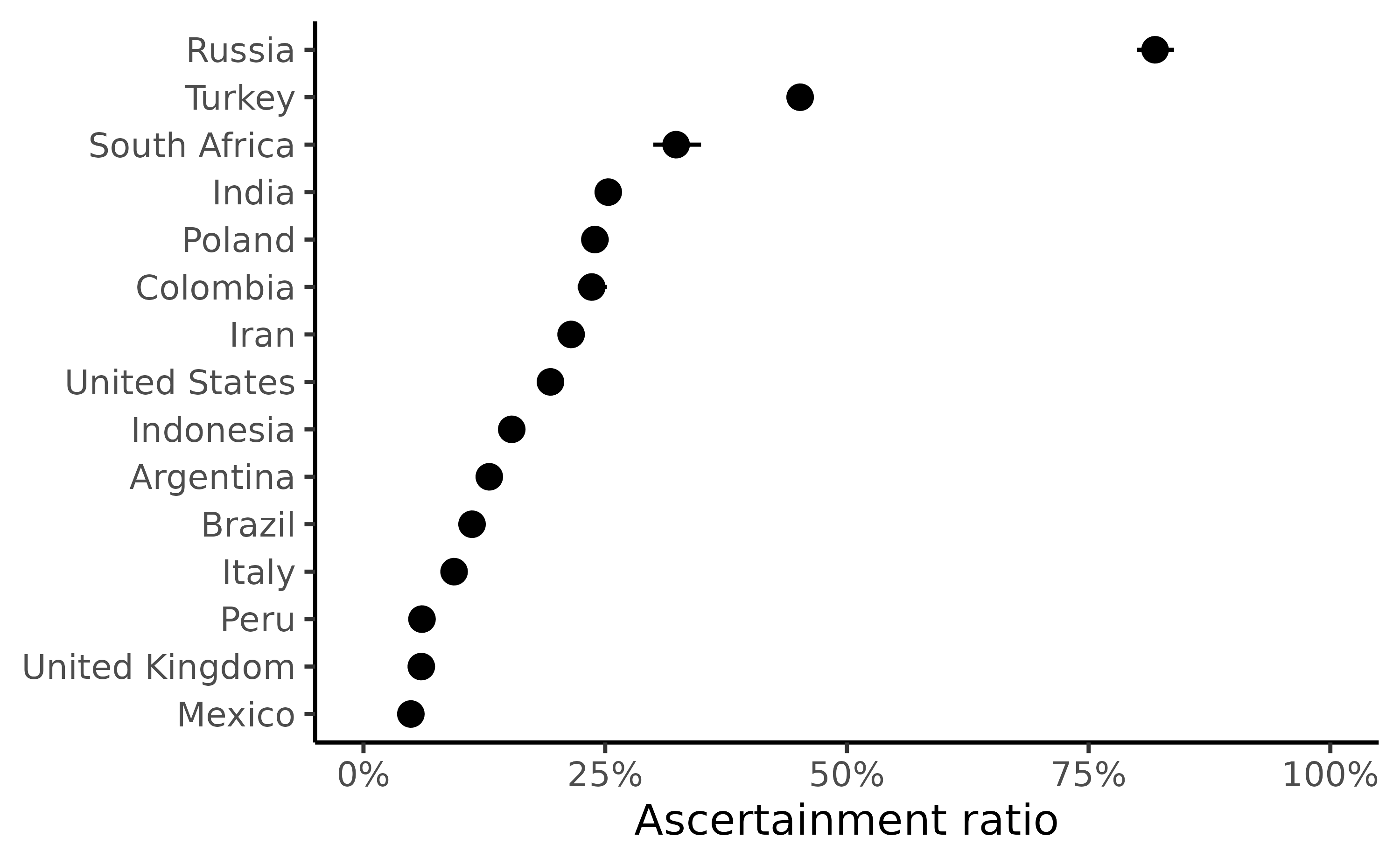

Figure 1: Example plot of the ascertainment ratio by country during the early stages of the Covid-19 pandemic.

References

Linton, Natalie M., Tetsuro Kobayashi, Yichi Yang, Katsuma Hayashi, Andrei R. Akhmetzhanov, Sung-mok Jung, Baoyin Yuan, Ryo Kinoshita, and Hiroshi Nishiura. 2020. “Incubation Period and Other Epidemiological Characteristics of 2019 Novel Coronavirus Infections with Right Truncation: A Statistical Analysis of Publicly Available Case Data.” Journal of Clinical Medicine 9 (2): 538. https://doi.org/10.3390/jcm9020538.

Verity, Robert, Lucy C. Okell, Ilaria Dorigatti, Peter Winskill, Charles Whittaker, Natsuko Imai, Gina Cuomo-Dannenburg, et al. 2020. “Estimates of the severity of coronavirus disease 2019: a model-based analysis.” The Lancet Infectious Diseases 20 (6): 669–77. https://doi.org/10.1016/S1473-3099(20)30243-7.