Estimating how disease severity varies over the course of an outbreak • cfr

The severity of a disease (commonly understood as the case fatality risk, CFR) might change during the course of an outbreak for multiple biological, epidemiological and behavioural reasons. cfr_time_varying() offers a convenient way to understand changes in disease severity over time using an approach with a finer time resolution that calculates severity over a moving time window, using methods from Nishiura et al. (2009).

New to calculating disease severity using cfr? You might want to see the “Get started” vignette first.

Use case

There are substantial changes to the characteristics of an outbreak over time — such as the introduction of therapeutics or a changing case definition. We want to estimate how disease severity in the form of the case fatality risk (CFR) changes over time while correcting for the delay in reporting the outcomes of cases.

What we have

A time-series of cases and deaths, (cases may be substituted by another indicator of infections over time);
Data on the distribution of delays, describing the probability an individual will die $t$ days after they were initially infected.

Potential reasons for changing disease severity

Change in the probability of infection being reported as a case,
Transmission dynamics within specific subgroups of differing risk of severe outcomes,
Introduction of vaccines or therapeutics reducing the relative risk of death,
Emergence of pathogen variants which may alter the mortality risk associated with infection.

library(cfr)

# packages to wrangle and plot data
library(dplyr)
library(tidyr)
library(purrr)
library(scales)
library(ggplot2)

Changing severity of the Covid-19 pandemic in the U.K.

This example shows time-varying severity estimation using cfr and data from the Covid-19 pandemic in the United Kingdom.

Preparing the raw data

We load example Covid-19 daily case and death data provided with the cfr package as covid_data, and subset for the first year of U.K. data.

We would expect the estimated CFR to change over this period due to changes in pandemic response policy, such as changes in case definitions, implementation and relaxation of lockdowns, and new variants emerging.

# get Covid data loaded with the package
data("covid_data")

# filter for the U.K
df_covid_uk <- filter(
  covid_data,
  country == "United Kingdom", date <= "2020-12-31"
)

# View the first few rows and recall necessary columns: date, cases, deaths
head(df_covid_uk)
#>         date        country cases deaths
#> 1 2020-01-03 United Kingdom     0      0
#> 2 2020-01-04 United Kingdom     0      0
#> 3 2020-01-05 United Kingdom     0      0
#> 4 2020-01-06 United Kingdom     0      0
#> 5 2020-01-07 United Kingdom     0      0
#> 6 2020-01-08 United Kingdom     0      0

Onset-to-death distribution for Covid-19

We retrieve the appropriate distribution of the duration between symptom onset and deaths reported in Linton et al. (2020); this is a lognormal distribution with $\mu$ = 2.577 and $\sigma$ = 0.440.

Linton et al. (2020) fitted a discrete lognormal distribution — but we use a continuous distribution here. See the vignette on delay distributions for more on when using a continuous instead of discrete distribution is acceptable, and on using discrete distributions with cfr.

Note also that we use the central estimates for each distribution parameter, and by ignoring uncertainty in these parameters the uncertainty in the resulting CFR is likely to be underestimated.

Estimating the naive and corrected CFR

We use the cfr_time_varying() function within the cfr package to calculate the time-varying CFR for the Covid-19 pandemic in the U.K., and plot the results.

The burn_in time is used to determine how many days at the start of the outbreak are excluded from the CFR calculation, potentially due to poor data quality at the beginning of an outbreak. The default value is 7, which ignores the first week of data.

The smoothing_window is used to smooth the case and death data using a rolling median with a window of the corresponding size (in days) using stats::runmed() internally — this is disabled by default. Users should apply smoothing if there are reporting artefacts such as lower reporting on weekends.

# calculating the naive time-varying CFR
df_covid_cfr_uk_naive <- cfr_time_varying(
  df_covid_uk,
  burn_in = 7,
  smoothing_window = 7
)

# calculating the corrected time-varying CFR
df_covid_cfr_uk_corrected <- cfr_time_varying(
  df_covid_uk,
  delay_density = function(x) dlnorm(x, meanlog = 2.577, sdlog = 0.440),
  burn_in = 7,
  smoothing_window = 7
)

# assign method tag and plot
df_covid_cfr_uk_naive$method <- "naive"
df_covid_cfr_uk_corrected$method <- "corrected"

df_covid_cfr_uk <- bind_rows(df_covid_cfr_uk_naive, df_covid_cfr_uk_corrected)

ggplot(df_covid_cfr_uk) +
  geom_ribbon(
    aes(
      x = date, ymin = severity_low, ymax = severity_high,
      fill = method
    ),
    alpha = 0.5
  ) +
  geom_line(
    aes(
      x = date, y = severity_estimate, colour = method
    )
  ) +
  scale_x_date(
    date_labels = "%b-%Y"
  ) +
  scale_y_continuous(
    labels = percent
  ) +
  scale_fill_brewer(
    palette = "Dark2",
    name = NULL,
    labels = c("Naive CFR", "Corrected CFR")
  ) +
  scale_colour_brewer(
    palette = "Dark2",
    name = NULL,
    labels = c("Naive CFR", "Corrected CFR")
  ) +
  labs(
    x = "Date", y = "CFR (%)"
  ) +
  coord_cartesian(
    expand = FALSE
  ) +
  theme_classic() +
  theme(legend.position = "top")
#> Warning: Removed 93 rows containing missing values or values outside the scale range
#> (`geom_line()`).

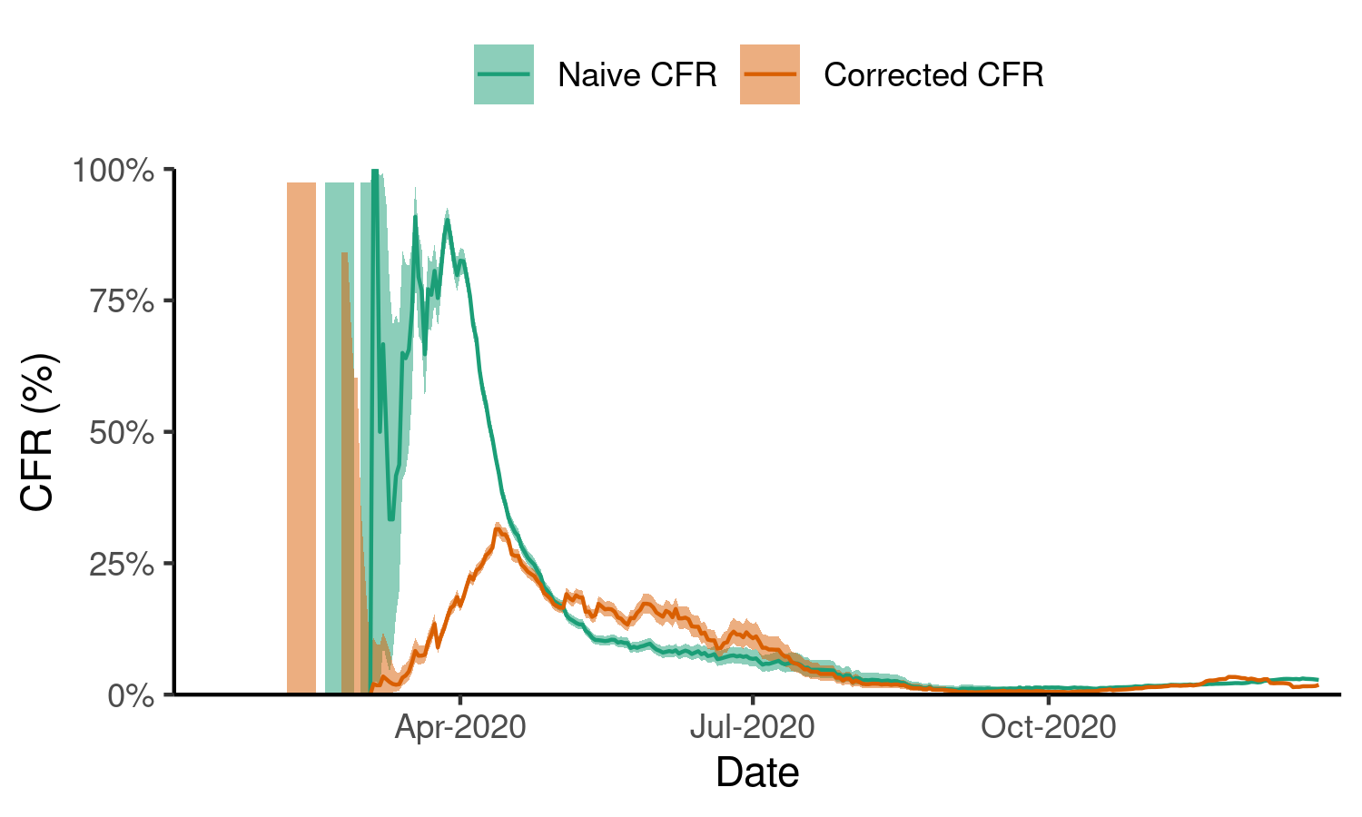
Example plot of the naive time-varying CFR. We calculate the time-varying CFR for the Covid-19 pandemic in the U.K., uncorrected for delays. The red line shows the CFR estimate while the shaded grey region shows the lower and upper limits of the estimate as 95% confidence intervals.

Note that the severity estimates and confidence intervals in cfr_time_varying() are obtained from a Binomial test on deaths (treated as ‘successes’) and estimated outcomes or cases (depending on whether delay correction is applied; treated as ‘trials’).

Severity of Covid-19 in multiple countries

cfr_time_varying() and other cfr functions can be conveniently applied over nested data to estimate the time-varying severity of Covid-19.

We refer the user to the book R for Data Science for a better explanation of some of the code used here, including from the packages in the Tidyverse.

We use the example Covid-19 cases and deaths data provided with the package as covid_data, while excluding four countries which only provide weekly data (with zeros for dates in between).

# countries with weekly reporting
weekly_reporting <- c("France", "Germany", "Spain", "Ukraine")
covid_data <- filter(covid_data, !country %in% weekly_reporting)

# for each country, get the time-varying severity estimate,
# correcting for delays and smoothing the case and death data

# first nest the data; nest() from {tidyr}
df_covid_cfr <- nest(
  covid_data,
  .by = country
)

# define delay density function
delay_density <- function(x) dlnorm(x, meanlog = 2.577, sdlog = 0.440)

# to each nested data frame, apply the function `cfr_time_varying`
# overwrite the `data` column, as all data will be preserved
df_covid_cfr <- mutate(
  df_covid_cfr,
  # using map() from {purrr}
  data = map(
    .x = data, .f = cfr_time_varying,
    # arguments to the function
    delay_density = delay_density,
    smoothing_window = 7, burn_in = 7
  )
)

# unnest the cfr data; unnest() from {tidyr}
df_covid_cfr <- unnest(df_covid_cfr, cols = data)

For simplicity, we use the same delay distribution between onset and death for all countries — users should note that this likely introduces biases given inter-country differences in testing or reporting policies.

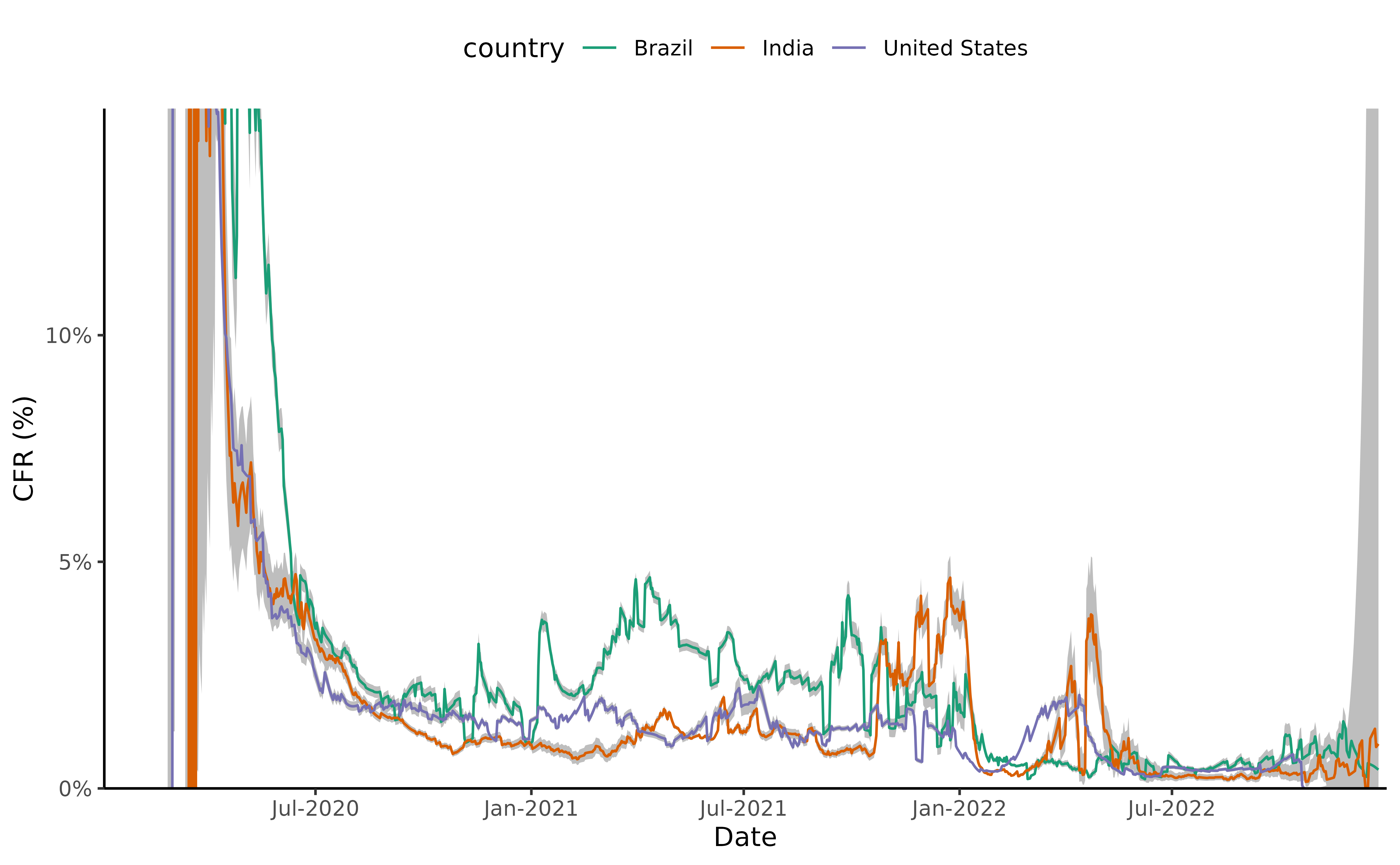
Finally we plot the time-varying CFR for a selection of three countries with large outbreaks of Covid-19: Brazil, India, and the United States.

filter(df_covid_cfr, country %in% c("Brazil", "India", "United States")) %>%
  ggplot() +
  geom_ribbon(
    aes(
      x = date, ymin = severity_low, ymax = severity_high,
      group = country
    ),
    fill = "grey"
  ) +
  geom_line(
    aes(
      x = date, y = severity_estimate, colour = country
    )
  ) +
  scale_x_date(
    date_labels = "%b-%Y"
  ) +
  scale_y_continuous(
    labels = percent
  ) +
  scale_colour_brewer(
    palette = "Dark2"
  ) +
  labs(
    x = "Date", y = "CFR (%)"
  ) +
  coord_cartesian(
    ylim = c(0, 0.15),
    expand = FALSE
  ) +
  theme_classic() +
  theme(legend.position = "top")
#> Warning: Removed 215 rows containing missing values or values outside the scale range
#> (`geom_line()`).

Example plot of the corrected time-varying CFR. We calculate the time-varying CFR for the Covid-19 pandemic in Brazil, India, and the United States, corrected for delays.

Details: Adjusting for delays between two time series

cfr_time_varying() estimates the number of cases which have a known outcome over time following Nishiura et al. (2009), by calculating a quantity $k_t$ for each day within the input data, which represents the number of cases with a known adverse outcome (usually death), on day $t$ .

$k_t = \sum_{j = 0}^t c_t f_{j - t}.$

We then assume that the severity measure (usually CFR) is binomially distributed in the following way

$$ d_t \sim {\sf Binomial}(k_t, \theta_t). $$

We use maximum likelihood estimation to determine the value of $\theta_t$ for each $t$ , where $\theta$ represents the severity measure of interest.

The precise severity measure — case fatality risk (CFR), infection fatality risk (IFR), hospitalisation fatality risk (HFR), etc. — that $\theta$ represents depends upon the input data given by the user.

Note that the function arguments burn_in and smoothing_window are not explicitly used in this calculation. burn_in controls how many estimates at the beginning of the outbreak are replaced with NAs — the calculation above is not applied to the first burn_in data points. The calculation is applied to the smoothed data, if a smoothing_window is specified.

References

Linton, Natalie M., Tetsuro Kobayashi, Yichi Yang, Katsuma Hayashi, Andrei R. Akhmetzhanov, Sung-mok Jung, Baoyin Yuan, Ryo Kinoshita, and Hiroshi Nishiura. 2020. “Incubation Period and Other Epidemiological Characteristics of 2019 Novel Coronavirus Infections with Right Truncation: A Statistical Analysis of Publicly Available Case Data.” Journal of Clinical Medicine 9 (2): 538. https://doi.org/10.3390/jcm9020538.

Nishiura, Hiroshi, Don Klinkenberg, Mick Roberts, and Johan A. P. Heesterbeek. 2009. “Early Epidemiological Assessment of the Virulence of Emerging Infectious Diseases: A Case Study of an Influenza Pandemic.” PLOS ONE 4 (8): e6852. https://doi.org/10.1371/journal.pone.0006852.