{epiparameter} Extraction Bias Analysis • epiparameter

If you are unfamiliar with the parameter extraction functionality in {epiparameter} the Conversion and Extraction vignette is a great place to start.

The {epiparameter} R package contains a set of functions to extract parameters of probability distributions given a set of summary statistics. These summary statistics can be the values at given percentiles of a distribution, or the median and range of a data set to which a distribution can be fit. Using these and specifying the distribution (e.g. gamma, lognormal, etc.) the parameters of the distribution can be extracted by optimisation using least-squares.

The precision and bias of this approach needs to be explored across the parameter space of the different distributions to understand potential erroneous inferences. This vignette aims to explore this inference bias for three distributions currently supported in {epiparameter} for parameter extraction: gamma, lognormal and Weibull. Extraction of parameters from a normal distribution is also supported in {epiparameter} but we do not test that in this vignette.

This is not an in depth analysis of the estimation methods implemented in {epiparameter}, but rather a supplementary article exploring the bias and precision of the functions. It is specific to the case of {epiparameter} and should not be taken as a generalisable result.

library(epiparameter)
library(ggplot2)

Extraction Bias

Extraction by percentiles

First we explore extraction from percentiles.

If a study reports the percentiles of a distribution, they are usually symmetrical (e.g. 5th and 95th, or 2.5th and 97.5th). However, in a few instances, only asymmetrical percentiles are available. We test whether asymmetry to varying degrees influences the bias of parameter extraction for all distributions.

We set up the parameter space to explore:

distributions <- c("gamma", "lnorm", "weibull")
dist_parameters <- seq(0.5, 2, 0.5)
lower_percentiles <- c(2.5, 5, 25, 40)
upper_percentiles <- c(60, 95, 97.5)

parameters_perc <- expand.grid(
  dist = distributions,
  param_1 = dist_parameters,
  param_2 = dist_parameters,
  lower = lower_percentiles,
  upper = upper_percentiles
)

# calculate the degree of asymmetry for each percentile combination
lw_interval_diff <- abs(0 - parameters_perc$lower)
up_interval_diff <- abs(100 - parameters_perc$upper)
deg_asym <- abs(lw_interval_diff - up_interval_diff)

# add degree of asymmetry to percentiles
parameters_perc <- cbind(parameters_perc, deg_asym)

# divide percentiles by 100 to make them probabilities for quantile functions
parameters_perc$lower <- parameters_perc$lower / 100
parameters_perc$upper <- parameters_perc$upper / 100

Now we can run the extraction for each point in parameter space. We set a seed to control for stochasticity when estimating the parameters, however changing or removing the seed should not drastically change the results or interpretation.

set.seed(1)

estim_params <- vector("list", nrow(parameters_perc))
# Loop through parameter space estimating parameters
for (params_idx in seq_len(nrow(parameters_perc))) {
  dist <- as.character(parameters_perc[params_idx, "dist"])
  percen <- unname(unlist(parameters_perc[params_idx, c("lower", "upper")]))

  if (dist == "lnorm") {
    true_values <- do.call(
      paste0("q", dist),
      list(
        p = percen,
        meanlog = parameters_perc[params_idx, "param_1"],
        sdlog = parameters_perc[params_idx, "param_2"]
      )
    )
  } else {
    true_values <- do.call(
      paste0("q", dist),
      list(
        p = percen,
        shape = parameters_perc[params_idx, "param_1"],
        scale = parameters_perc[params_idx, "param_2"]
      )
    )
  }

  # message about stochastic optimisation suppressed
  estim_params[[params_idx]] <- suppressMessages(
    extract_param(
      type = "percentiles",
      values = true_values,
      distribution = dist,
      percentiles = percen
    )
  )
}

# combine results
results <- cbind(parameters_perc, do.call(rbind, estim_params))

colnames(results) <- c(
  "dist", "param_1", "param_2", "lower", "upper",
  "deg_asym", "estim_param_1", "estim_param_2"
)

# calculate absolute difference between true parameter and estimated value
results <- cbind(
  results,
  diff_param_1 = abs(results$param_1 - results$estim_param_1),
  diff_param_2 = abs(results$param_2 - results$estim_param_2)
)

The extract_param() function re-runs the optimisation until convergence to a set tolerance is achieved (or a maximum number of iterations is reached) to more reliably return the global optimum. In theory, this should help to minimise bias and instability in the parameter estimation. See the function documentation (?extract_param()) or the Conversion and Extraction vignette for more details.

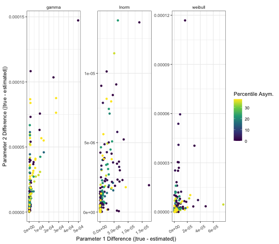
The extraction bias can be explored:

# plot differences by distribution
ggplot(data = results) +
  geom_point(mapping = aes(
    x = diff_param_1,
    y = diff_param_2,
    colour = deg_asym
  )) +
  scale_x_continuous(name = "Parameter 1 Difference (|true - estimated|)") +
  scale_y_continuous(name = "Parameter 2 Difference (|true - estimated|)") +
  labs(colour = "Percentile Asym.") +
  theme_bw() +
  scale_color_viridis_c() +
  facet_wrap(facets = vars(dist), scales = "free") +
  theme(
    strip.background = element_blank(),
    axis.text.x = element_text(angle = 30, vjust = 0.5)
  )

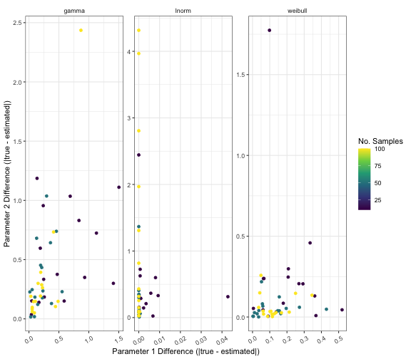
Parameter estimation bias facetted by distribution. Parameter 1 is either the shape parameter, for gamma and Weibull distributions, or meanlog for the lognormal distribution. Parameter 2 is either the scale parameter for gamma and Weibull distributions, or sdlog for the lognormal distribution.

Extraction by median and range

The same analysis as above can be repeated, this time using the other summary statistic possibly reported in studies: median and range of data. For this extraction the number of samples used to infer the distribution is required as this can impact the possible range exhibited by the data.

Set up the parameter space:

n_samples <- c(10, 50, 100)
parameters_range <- expand.grid(
  dist = distributions, # same as above
  param_1 = dist_parameters, # same as above
  param_2 = dist_parameters, # same as above
  n_samples = n_samples
)

estim_params <- vector("list", nrow(parameters_range))
# Loop through parameter space estimating parameters
for (params_idx in seq_len(nrow(parameters_range))) {
  dist <- as.character(parameters_range[params_idx, "dist"])
  n_samples <- parameters_range[params_idx, "n_samples"]
  # while loop to ensure values are min < median < max
  resample_values <- TRUE
  while (resample_values) {
    if (dist == "lnorm") {
      true_median <- do.call(
        paste0("q", dist),
        list(
          p = 0.5,
          meanlog = parameters_range[params_idx, "param_1"],
          sdlog = parameters_range[params_idx, "param_2"]
        )
      )
      true_range <- do.call(
        paste0("r", dist),
        list(
          n = n_samples,
          meanlog = parameters_range[params_idx, "param_1"],
          sdlog = parameters_range[params_idx, "param_2"]
        )
      )
      true_range <- c(min(true_range), max(true_range))
    } else {
      true_median <- do.call(
        paste0("q", dist),
        list(
          p = 0.5,
          shape = parameters_range[params_idx, "param_1"],
          scale = parameters_range[params_idx, "param_2"]
        )
      )
      true_range <- do.call(
        paste0("r", dist),
        list(
          n = n_samples,
          shape = parameters_range[params_idx, "param_1"],
          scale = parameters_range[params_idx, "param_2"]
        )
      )
      true_range <- c(min(true_range), max(true_range))
    }
    true_values <- c(true_median, true_range)
    if (true_values[2] < true_values[1] && true_values[1] < true_values[3]) {
      resample_values <- FALSE
    }
  }
  # message about stochastic optimisation suppressed
  estim_params[[params_idx]] <- suppressMessages(
    expr = extract_param(
      type = "range",
      values = true_values,
      distribution = dist,
      samples = n_samples
    )
  )
}
#> Warning: Maximum optimisation iterations reached, returning result early. 
#> Result may not be reliable.


# combine results
results <- cbind(parameters_range, do.call(rbind, estim_params))

colnames(results) <- c(
  "dist", "param_1", "param_2", "n_samples", "estim_param_1", "estim_param_2"
)

# calculate absolute difference between true parameter and estimated value
results <- cbind(
  results,
  diff_param_1 = abs(results$param_1 - results$estim_param_1),
  diff_param_2 = abs(results$param_2 - results$estim_param_2)
)

Plot results:

# plot differences by distribution
ggplot(data = results) +
  geom_point(
    mapping = aes(
      x = diff_param_1,
      y = diff_param_2,
      colour = n_samples
    )
  ) +
  scale_x_continuous(name = "Parameter 1 Difference (|true - estimated|)") +
  scale_y_continuous(name = "Parameter 2 Difference (|true - estimated|)") +
  labs(colour = "No. Samples") +
  theme_bw() +
  scale_color_viridis_c() +
  facet_wrap(facets = vars(dist), scales = "free") +
  theme(
    strip.background = element_blank(),
    axis.text.x = element_text(angle = 30, vjust = 0.5)
  )

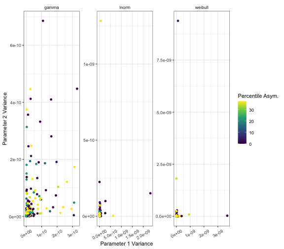
Parameter extraction bias. Parameter 1 is either the shape parameter, for gamma and Weibull distributions, or meanlog for the lognormal distribution. Parameter 2 is either the scale parameter for gamma and Weibull distributions, or sdlog for the lognormal distribution.

Extraction precision

Extraction by percentiles

The two analyses above used a single extraction (replicate), however, it may be that the estimation of the parameters is unstable for a given set of percentiles or median range. Therefore, we finish with a test of whether repeated extraction of parameters from a single percentile has large variance which would indicate the parameter extraction is unstable, imprecise, and potentially untrustworthy.

We use the same parameter space for percentiles as defined above (parameters_perc). Now we can run the extraction for a set of replicates to compute the variance of parameter estimates over those replicates.

estim_param_var <- vector("list", nrow(parameters_perc))
# Loop through parameter space estimating parameters
for (params_idx in seq_len(nrow(parameters_perc))) {
  dist <- as.character(parameters_perc[params_idx, "dist"])
  percen <- unname(unlist(parameters_perc[params_idx, c("lower", "upper")]))

  if (dist == "lnorm") {
    true_values <- do.call(
      paste0("q", dist),
      list(
        p = percen,
        meanlog = parameters_perc[params_idx, "param_1"],
        sdlog = parameters_perc[params_idx, "param_2"]
      )
    )
  } else {
    true_values <- do.call(
      paste0("q", dist),
      list(
        p = percen,
        shape = parameters_perc[params_idx, "param_1"],
        scale = parameters_perc[params_idx, "param_2"]
      )
    )
  }

  # message about stochastic optimisation suppressed
  estim <- suppressMessages(
    replicate(
      n = 5,
      expr = extract_param(
        type = "percentiles",
        values = true_values,
        distribution = dist,
        percentiles = percen
      )
    )
  )
  estim_param_var[[params_idx]] <- apply(estim, MARGIN = 1, FUN = var)
}

# combine results
results <- cbind(parameters_perc, do.call(rbind, estim_param_var))

colnames(results) <- c(
  "dist", "param_1", "param_2", "lower", "upper",
  "deg_asym", "estim_param_1_var", "estim_param_2_var"
)

ggplot(data = results) +
  geom_point(mapping = aes(
    x = estim_param_1_var,
    y = estim_param_2_var,
    colour = deg_asym
  )) +
  scale_x_continuous(name = "Parameter 1 Variance") +
  scale_y_continuous(name = "Parameter 2 Variance") +
  labs(colour = "Percentile Asym.") +
  theme_bw() +
  scale_color_viridis_c() +
  facet_wrap(facets = vars(dist), scales = "free") +
  theme(
    strip.background = element_blank(),
    axis.text.x = element_text(angle = 30, vjust = 0.5)
  )

Parameter extraction precision, facetted by distribution. Parameter 1 is either the shape parameter, for gamma and Weibull distributions, or meanlog for the lognormal distribution. Parameter 2 is either the scale parameter for gamma and Weibull distributions, or sdlog for the lognormal distribution.

Extraction by median and range

The same test of estimation precision can be performed for the extraction from median and range.

estim_param_var <- vector("list", nrow(parameters_range))
# Loop through parameter space estimating parameters
for (params_idx in seq_len(nrow(parameters_range))) {
  dist <- as.character(parameters_range[params_idx, "dist"])
  n_samples <- parameters_range[params_idx, "n_samples"]

  # while loop to ensure values are min < median < max
  resample_values <- TRUE
  while (resample_values) {
    if (dist == "lnorm") {
      true_median <- do.call(
        paste0("q", dist),
        list(
          p = 0.5,
          meanlog = parameters_range[params_idx, "param_1"],
          sdlog = parameters_range[params_idx, "param_2"]
        )
      )
      true_range <- do.call(
        paste0("r", dist),
        list(
          n = n_samples,
          meanlog = parameters_range[params_idx, "param_1"],
          sdlog = parameters_range[params_idx, "param_2"]
        )
      )
      true_range <- c(min(true_range), max(true_range))
    } else {
      true_median <- do.call(
        paste0("q", dist),
        list(
          p = 0.5,
          shape = parameters_range[params_idx, "param_1"],
          scale = parameters_range[params_idx, "param_2"]
        )
      )
      true_range <- do.call(
        paste0("r", dist),
        list(
          n = n_samples,
          shape = parameters_range[params_idx, "param_1"],
          scale = parameters_range[params_idx, "param_2"]
        )
      )
      true_range <- c(min(true_range), max(true_range))
    }
    true_values <- c(true_median, true_range)
    if (true_values[2] < true_values[1] && true_values[1] < true_values[3]) {
      resample_values <- FALSE
    }
  }
  # message about stochastic optimisation suppressed
  estim <- suppressMessages(
    replicate(
      n = 5,
      expr = extract_param(
        type = "range",
        values = true_values,
        distribution = dist,
        samples = n_samples
      )
    )
  )
  estim_param_var[[params_idx]] <- apply(estim, MARGIN = 1, FUN = var)
}
#> Warning: Maximum optimisation iterations reached, returning result early. 
#> Result may not be reliable.


# combine results
results <- cbind(parameters_range, do.call(rbind, estim_param_var))

colnames(results) <- c(
  "dist", "param_1", "param_2", "n_samples", "estim_param_1_var",
  "estim_param_2_var"
)

ggplot(data = results) +
  geom_point(mapping = aes(
    x = estim_param_1_var,
    y = estim_param_2_var,
    colour = n_samples
  )) +
  scale_x_continuous(name = "Parameter 1 Variance") +
  scale_y_continuous(name = "Parameter 2 Variance") +
  labs(colour = "No. Samples") +
  theme_bw() +
  scale_color_viridis_c() +
  facet_wrap(facets = vars(dist), scales = "free") +
  theme(
    strip.background = element_blank(),
    axis.text.x = element_text(angle = 30, vjust = 0.5)
  )

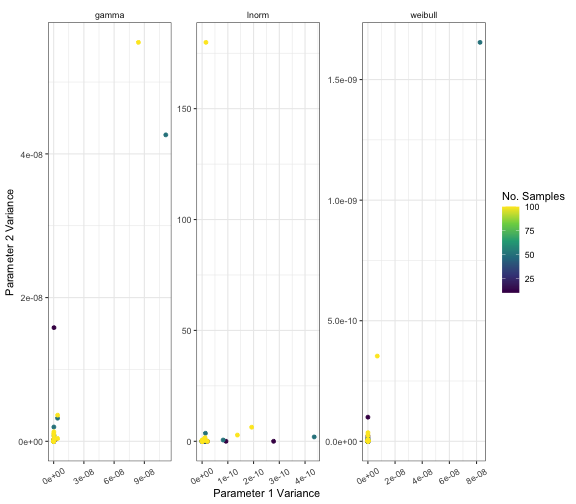
From the plots in this vignette, the bias is low and precision is high when extracting parameters from the gamma, lognormal and Weibull distributions from both percentiles of the distribution and from median and range of a data set.

The asymmetry of percentiles and sample size of the data does not noticeably influence the bias in parameter extraction.

However, this does not ensure reliable extract for all use cases of the extract_param() function and we recommend checking the output for spurious results.