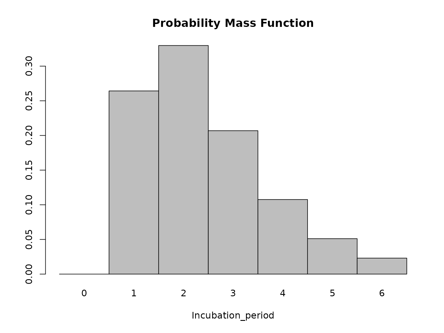
Plot an <epiparameter> object by displaying the either the
probability mass function (PMF), (in the case of discrete distributions)
or probability density function (PDF) (in the case of continuous
distributions), or the cumulative distribution function (CDF).
Usage
# S3 method for class 'epiparameter'
plot(x, cumulative = FALSE, ...)Details
By default if the xlim argument is not specified the distribution is
plotted between day 0 and the 99th quantile of the distribution.
Alternatively, a numeric vector of length 2 with the
first and last day to plot on the x-axis can be supplied to xlim
(through ...).
Examples
# plot continuous epiparameter
ep <- epiparameter(
  disease = "ebola",
  epi_name = "incubation_period",
  prob_distribution = create_prob_distribution(
    prob_distribution = "gamma",
    prob_distribution_params = c(shape = 2, scale = 1)
  )
)
#> Citation cannot be created as author, year, journal or title is missing
plot(ep)


# plot different day range (x-axis)
plot(ep, xlim = c(0, 10))


# plot CDF
plot(ep, cumulative = TRUE)


# plot discrete epiparameter
ep <- discretise(ep)
plot(ep)

