Time-varying case fatality risk • simulist

If you are unfamiliar with the {simulist} package or the sim_linelist() function Get Started vignette is a great place to start.

This vignette demonstrates how to simulate line list data using the time-varying case fatality risk and gives an overview of the methodological details.

The {simulist} R package uses an individual-based branching process simulation to generate contacts and cases for line list and contact tracing data. The time-varying case fatality risk feature provides a way to incorporate aspects of epidemics where the risk of death may decrease through time, potentially due to improved medical treatment, vaccination or viral evolution. It is also possible to model increasing case fatality risk through time, or a stepwise risk function where the risk of death shifts between states.

The time-varying case fatality risk implemented in this package is not meant to explicitly model these factors, but rather to give the user an option to more closely resemble fatality risk through the course of an epidemic, possibly because there is data on this, or just to simulate data that has these characteristics.

See the {epidemics} R package for a population-level epidemic simulation package with explicit interventions and vaccinations.

Given that setting a time-varying case fatality risk is not needed for most use cases of the {simulist} R package, this feature uses the config argument in the sim_*() functions. Therefore, the time-varying case fatality risk can be set when calling create_config() (see below for details).

library(simulist)
library(epiparameter)
library(tidyr)
library(dplyr)
#> 
#> Attaching package: 'dplyr'
#> The following objects are masked from 'package:stats':
#> 
#>     filter, lag
#> The following objects are masked from 'package:base':
#> 
#>     intersect, setdiff, setequal, union
library(incidence2)
#> Loading required package: grates
library(ggplot2)

First we will demonstrate the default setting of a constant case fatality risk throughout an epidemic.

We load the required delay distributions using the {epiparameter} package, by either manually creating them (contact distribution and infectious period), or load them from the {epiparameter} library of epidemiological parameters (onset-to-hospitalisation and onset-to-death).

contact_distribution <- epiparameter(
  disease = "COVID-19",
  epi_dist = "contact distribution",
  prob_distribution = "pois",
  prob_distribution_params = c(mean = 2)
)
#> Citation cannot be created as author, year, journal or title is missing

infectious_period <- epiparameter(
  disease = "COVID-19",
  epi_dist = "infectious period",
  prob_distribution = "gamma",
  prob_distribution_params = c(shape = 3, scale = 3)
)
#> Citation cannot be created as author, year, journal or title is missing

# get onset to hospital admission from {epiparameter} database
onset_to_hosp <- epiparameter_db(
  disease = "COVID-19",
  epi_dist = "onset to hospitalisation",
  single_epiparameter = TRUE
)
#> Using Linton N, Kobayashi T, Yang Y, Hayashi K, Akhmetzhanov A, Jung S, Yuan
#> B, Kinoshita R, Nishiura H (2020). "Incubation Period and Other
#> Epidemiological Characteristics of 2019 Novel Coronavirus Infections
#> with Right Truncation: A Statistical Analysis of Publicly Available
#> Case Data." _Journal of Clinical Medicine_. doi:10.3390/jcm9020538
#> <https://doi.org/10.3390/jcm9020538>.. 
#> To retrieve the citation use the 'get_citation' function

# get onset to death from {epiparameter} database
onset_to_death <- epiparameter_db(
  disease = "COVID-19",
  epi_dist = "onset to death",
  single_epiparameter = TRUE
)
#> Using Linton N, Kobayashi T, Yang Y, Hayashi K, Akhmetzhanov A, Jung S, Yuan
#> B, Kinoshita R, Nishiura H (2020). "Incubation Period and Other
#> Epidemiological Characteristics of 2019 Novel Coronavirus Infections
#> with Right Truncation: A Statistical Analysis of Publicly Available
#> Case Data." _Journal of Clinical Medicine_. doi:10.3390/jcm9020538
#> <https://doi.org/10.3390/jcm9020538>.. 
#> To retrieve the citation use the 'get_citation' function

We set the seed to ensure we have the same output each time the vignette is rendered. When using {simulist}, setting the seed is not required unless you need to simulate the same line list multiple times.

set.seed(1)

Constant case fatality risk

When calling the create_config() function the default output contains a list element named time_varying_death_risk set to NULL. This corresponds to a constant case fatality risk over time, which is controlled by the hosp_death_risk and non_hosp_death_risk arguments. The defaults for these two arguments are:

death risk when hospitalised (hosp_death_risk): 0.5 (50%)
death risk outside of hospitals (non_hosp_death_risk): 0.05 (5%)

In this example we set them explicitly to be clear which risks we’re using, but otherwise the hosp_death_risk, non_hosp_death_risk and config do not need to be specified and can use their default values.

For all examples in this vignette we will set the epidemic size to be between 500 and 1,000 cases, to ensure that we can clearly see the case fatality patterns in the data.

See the Get Started vignette section on Controlling Outbreak Size for more information on this.

linelist <- sim_linelist(
  contact_distribution = contact_distribution,
  infectious_period = infectious_period,
  prob_infection = 0.5,
  onset_to_hosp = onset_to_hosp,
  onset_to_death = onset_to_death,
  hosp_death_risk = 0.5,
  non_hosp_death_risk = 0.05,
  outbreak_size = c(500, 1000),
  config = create_config()
)

# first 6 rows of linelist
head(linelist)
#>   id        case_name case_type sex age date_onset date_admission   outcome
#> 1  1       Mark Allen suspected   m  60 2023-01-01           <NA> recovered
#> 2  2    Emma Kirscher  probable   f  54 2023-01-04           <NA> recovered
#> 3  4     James Coyote confirmed   m  12 2023-01-05           <NA> recovered
#> 4  6 Dagoberto Medina  probable   m  45 2023-01-07           <NA> recovered
#> 5  7  Sundus al-Malek confirmed   f  11 2023-01-09           <NA> recovered
#> 6  8  Andrew Billings  probable   m  36 2023-01-08           <NA> recovered
#>   date_outcome date_first_contact date_last_contact ct_value
#> 1         <NA>               <NA>              <NA>       NA
#> 2         <NA>         2023-01-03        2023-01-06       NA
#> 3         <NA>         2022-12-30        2023-01-02     25.3
#> 4         <NA>         2023-01-03        2023-01-06       NA
#> 5         <NA>         2023-01-01        2023-01-05     25.3
#> 6         <NA>         2023-01-01        2023-01-05       NA

To visualise the incidence of cases and deaths over time we will use the {incidence2} R package.

For more information on using {incidence2} to plot line list data see the Visualising simulated data vignette.

Before converting the line list <data.frame> to an <incidence> object we need to ungroup the outcome columns into their own columns using the {tidyr} and {dplyr} R packages from the Tidyverse.

linelist <- linelist %>%
  pivot_wider(
    names_from = outcome,
    values_from = date_outcome
  ) %>%
  rename(
    date_death = died,
    date_recovery = recovered
  )

daily <- incidence(
  linelist,
  date_index = c(
    onset = "date_onset",
    death = "date_death"
  ),
  interval = "daily"
)
daily <- complete_dates(daily)
plot(daily)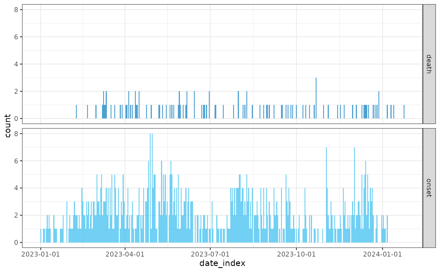

Daily incidence of cases from symptom onset and incidence of deaths. Case fatality risk for hospitalised individuals is 0.5 and the risk for non-hospitalised individuals is 0.05, and these risks are constant through time.

Higher risk of case fatality

We repeat the above simulation but increase the risk of case fatality for both hospitalised (hosp_death_risk) and non-hospitalised (non_hosp_death_risk) individuals infected.

linelist <- sim_linelist(
  contact_distribution = contact_distribution,
  infectious_period = infectious_period,
  prob_infection = 0.5,
  onset_to_hosp = onset_to_hosp,
  onset_to_death = onset_to_death,
  hosp_death_risk = 0.9,
  non_hosp_death_risk = 0.75,
  outbreak_size = c(500, 1000),
  config = create_config()
)
#> Warning: Number of cases exceeds maximum outbreak size. 
#> Returning data early with 1026 cases and 1994 total contacts (including cases).

head(linelist)
#>   id        case_name case_type sex age date_onset date_admission   outcome
#> 1  1     Brian Cabral suspected   m  42 2023-01-01     2023-01-10 recovered
#> 2  2         Noah Han confirmed   m  25 2023-01-06     2023-01-12      died
#> 3  4 Jessenia Bechtel confirmed   f  64 2023-01-07           <NA>      died
#> 4  6   Ilhaam al-Azam confirmed   f  46 2023-01-09           <NA> recovered
#> 5  8   Yasmine Turner  probable   f  78 2023-01-08           <NA>      died
#> 6 10 Amaani al-Akbari  probable   f  13 2023-01-15           <NA>      died
#>   date_outcome date_first_contact date_last_contact ct_value
#> 1         <NA>               <NA>              <NA>       NA
#> 2   2023-02-26         2022-12-29        2023-01-03     24.4
#> 3   2023-02-04         2023-01-05        2023-01-07     24.4
#> 4         <NA>         2023-01-09        2023-01-11     24.4
#> 5   2023-02-07         2023-01-08        2023-01-09       NA
#> 6   2023-02-17         2023-01-07        2023-01-11       NA

linelist <- linelist %>%
  pivot_wider(
    names_from = outcome,
    values_from = date_outcome
  ) %>%
  rename(
    date_death = died,
    date_recovery = recovered
  )

daily <- incidence(
  linelist,
  date_index = c(
    onset = "date_onset",
    death = "date_death"
  ),
  interval = "daily"
)
daily <- complete_dates(daily)
plot(daily)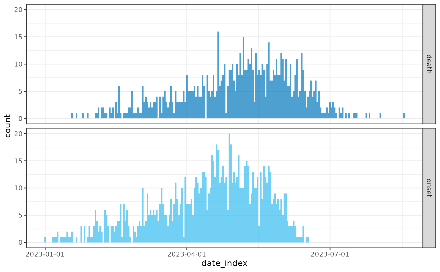

Daily incidence of cases from symptom onset and incidence of deaths. Case fatality risk for hospitalised individuals is 0.9 and the risk for non-hospitalised individuals is 0.75, and these risks are constant through time.

Continuous time-varying case fatality risk

Now we’ve seen what the constant case fatality risk simulations look like, we can simulate with a time-varying function for the risk.

This is setup by calling the create_config() function, and providing an anonymous function with two arguments, risk and time, to time_varying_death_risk. This function will then use the relevant risk (e.g. hosp_death_risk) and the time an individual is infected and calculates the probability (or risk) of death.

The create_config() function has no named arguments, and the argument you are modifying needs to be matched by name exactly (case sensitive). See ?create_config() for documentation.

config <- create_config(
  time_varying_death_risk = function(risk, time) risk * exp(-0.05 * time)
)

Here we set the case fatality risk to exponentially decrease through time. This will provide a shallow (monotonic) decline of case fatality through the simulated epidemic.

exp_df <- data.frame(
  time = 1:150,
  value = config$time_varying_death_risk(risk = 0.9, time = 1:150)
)
ggplot(exp_df) +
  geom_point(mapping = aes(x = time, y = value)) +
  scale_y_continuous(name = "Value") +
  scale_x_continuous(name = "Time (Days)") +
  theme_bw()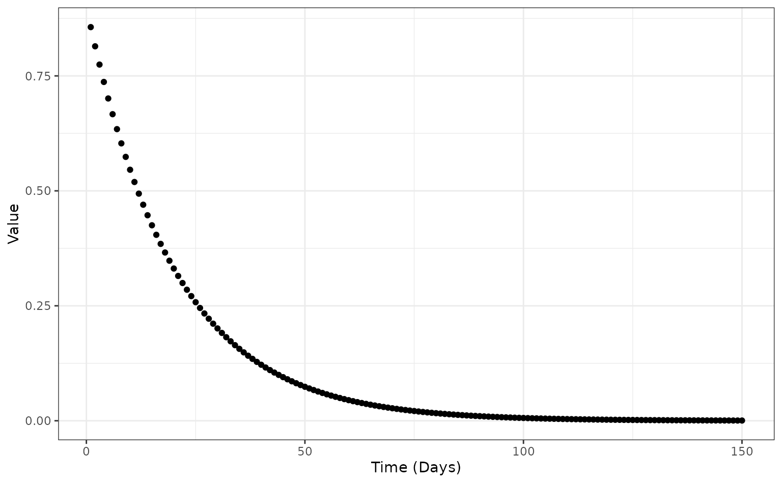

The time-varying hospitalised case fatality risk function (config$time_varying_death_risk) throughout the epidemic. In this case the hospitalised risks (hosp_death_risk) are at their maximum value at day 0 and decline through time, with risk approaching zero at around day 100.

Advanced

The time-varying case fatality risk function modifies the the death risk specified by hosp_death_risk and non_hosp_death_risk. In this example, the user-supplied hosp_death_risk and non_hosp_death_risk are the maximum values, because the user-supplied time-varying function is declining over time, however, a user-supplied function may also increase over time, or fluctuate. The requirements are that the time-varying case fatality risk for both hospitalised and non-hospitalised infections must be between 0 and 1, otherwise the function will error.

In the example below hosp_death_risk is 0.9 and non_hosp_death_risk is 0.75, and the time-varying case fatality risk function is an exponential decline. This means that on day 0 of the epidemic (i.e. first infection seeds the outbreak) the risks will be 0.9 and 0.75. But any time after the start of the epidemic ( $t_0 + \Delta t$ ) the risks will be lower, and when the exponential function approaches zero the risk of a case dying will also go to zero.

Simulating with the time-varying case fatality risk:

linelist <- sim_linelist(
  contact_distribution = contact_distribution,
  infectious_period = infectious_period,
  prob_infection = 0.5,
  onset_to_hosp = onset_to_hosp,
  onset_to_death = onset_to_death,
  hosp_death_risk = 0.9,
  non_hosp_death_risk = 0.75,
  outbreak_size = c(500, 1000),
  config = config
)

head(linelist)
#>   id         case_name case_type sex age date_onset date_admission   outcome
#> 1  1       Jacob Swope confirmed   m  57 2023-01-01           <NA>      died
#> 2  3     Raeven Tipton  probable   f   7 2023-01-04           <NA>      died
#> 3  4         Seung Chu suspected   f  34 2023-01-07           <NA> recovered
#> 4  5  Shaahir el-Pasha confirmed   m  34 2023-01-04           <NA>      died
#> 5  6 Hibbaan el-Hammad suspected   m  64 2023-01-05           <NA>      died
#> 6  8         Troy Yang confirmed   m  41 2023-01-14           <NA>      died
#>   date_outcome date_first_contact date_last_contact ct_value
#> 1   2023-01-08               <NA>              <NA>     25.9
#> 2   2023-01-29         2022-12-31        2023-01-03       NA
#> 3         <NA>         2022-12-29        2023-01-02       NA
#> 4   2023-01-18         2023-01-01        2023-01-05     25.9
#> 5   2023-02-06         2023-01-07        2023-01-08       NA
#> 6   2023-02-06         2023-01-11        2023-01-13     25.9

linelist <- linelist %>%
  pivot_wider(
    names_from = outcome,
    values_from = date_outcome
  ) %>%
  rename(
    date_death = died,
    date_recovery = recovered
  )

daily <- incidence(
  linelist,
  date_index = c(
    onset = "date_onset",
    death = "date_death"
  ),
  interval = "daily"
)
daily <- complete_dates(daily)
plot(daily)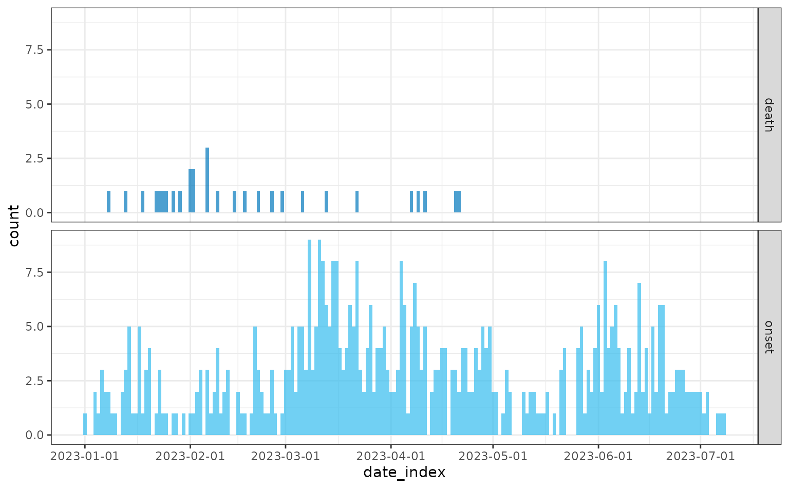

Daily incidence of cases from symptom onset and incidence of deaths. The baseline case fatality risk for hospitalised individuals is 0.9 and for non-hospitalised individuals is 0.75, and these decline exponentially through time.

Stepwise time-varying case fatality risk

In addition to a continuously varying case fatality risk function, the simulation can also work with stepwise (or piecewise) functions. This is where the risk will instantaneously change at a given point in time to another risk level.

To achieve this, we again specify an anonymous function in create_config(), but have the risk of a case dying set as the baseline hosp_death_risk and non_hosp_death_risk for the first 60 days of the outbreak and then become zero (i.e. if an individual is infected after day 60 they will definitely recover).

config <- create_config(
  time_varying_death_risk = function(risk, time) ifelse(test = time < 60, yes = risk, no = 0)
)

stepwise_df <- data.frame(
  time = 1:150,
  value = config$time_varying_death_risk(risk = 0.9, time = 1:150)
)
ggplot(stepwise_df) +
  geom_point(mapping = aes(x = time, y = value)) +
  scale_y_continuous(name = "Value") +
  scale_x_continuous(name = "Time (Days)") +
  theme_bw()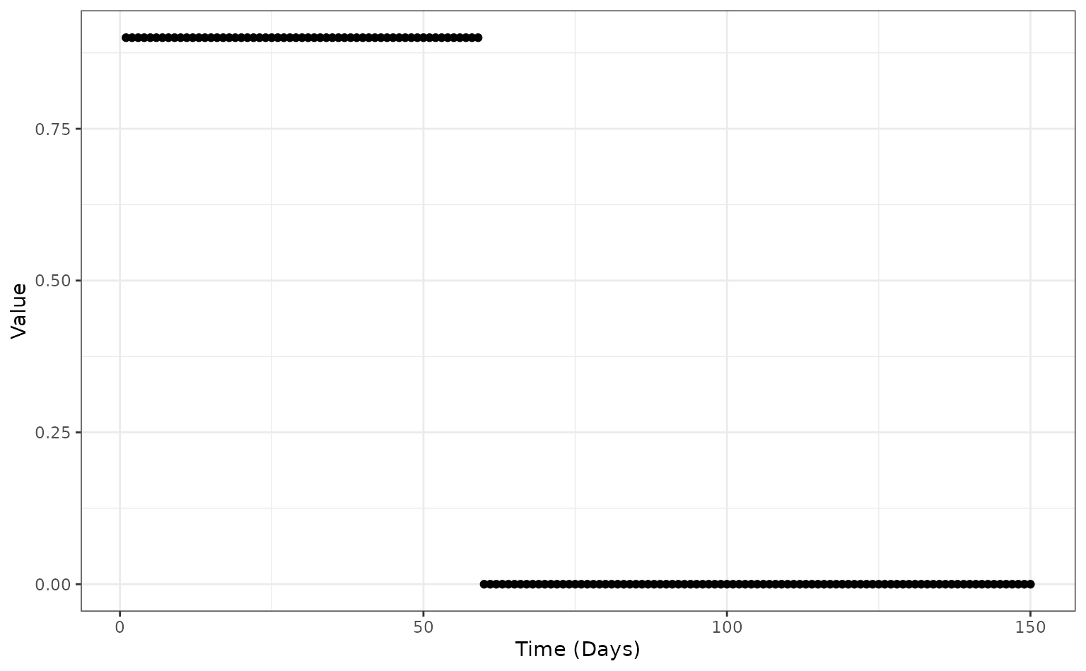

The time-varying case fatality risk function (config$time_varying_death_risk) for the hospitalised death risk (hosp_death_risk) and non-hospitalised death risk (non_hosp_death_risk) throughout the epidemic. In this case the risks are at their user-supplied values from day 0 to day 60, and then become 0 onwards.

Simulating with the stepwise time-varying case fatality risk:

linelist <- sim_linelist(
  contact_distribution = contact_distribution,
  infectious_period = infectious_period,
  prob_infection = 0.5,
  onset_to_hosp = onset_to_hosp,
  onset_to_death = onset_to_death,
  hosp_death_risk = 0.9,
  non_hosp_death_risk = 0.75,
  outbreak_size = c(500, 1000),
  config = config
)
#> Warning: Number of cases exceeds maximum outbreak size. 
#> Returning data early with 1010 cases and 1987 total contacts (including cases).

head(linelist)
#>   id        case_name case_type sex age date_onset date_admission   outcome
#> 1  1      Adam Bettis suspected   m  10 2023-01-01     2023-01-02      died
#> 2  2         Sean Tat confirmed   m  36 2023-01-02     2023-01-05      died
#> 3  4   Menandez Walck suspected   m  48 2023-01-02           <NA> recovered
#> 4  6     Marcel Jones suspected   m  25 2023-01-06           <NA> recovered
#> 5  7   Adriana Merino  probable   f  29 2023-01-07           <NA>      died
#> 6  9 Ubaida al-Khalid confirmed   m  83 2023-01-18           <NA> recovered
#>   date_outcome date_first_contact date_last_contact ct_value
#> 1   2023-02-06               <NA>              <NA>       NA
#> 2   2023-01-25         2023-01-02        2023-01-05     26.9
#> 3         <NA>         2023-01-05        2023-01-06       NA
#> 4         <NA>         2022-12-31        2023-01-03       NA
#> 5   2023-01-13         2023-01-04        2023-01-05       NA
#> 6         <NA>         2023-01-01        2023-01-04     26.9

linelist <- linelist %>%
  pivot_wider(
    names_from = outcome,
    values_from = date_outcome
  ) %>%
  rename(
    date_death = died,
    date_recovery = recovered
  )

daily <- incidence(
  linelist,
  date_index = c(
    onset = "date_onset",
    death = "date_death"
  ),
  interval = "daily"
)
daily <- complete_dates(daily)
plot(daily)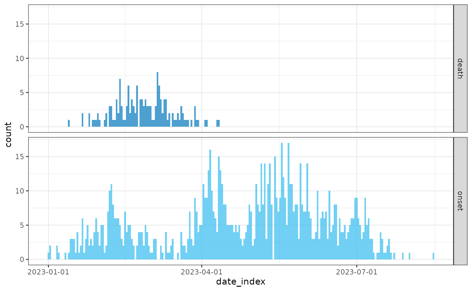

Daily incidence of cases from symptom onset and incidence of deaths. The maximum case fatality risk for hospitalised individuals is 0.9 and for non-hospitalised individuals is 0.75, and these rates remain constant from days 0 to 60, and then go to 0 from day 60 onwards.

The same stepwise function can also be used to specify time windows were the risk of death is reduced. Here we specify the hosp_death_risk and non_hosp_death_risk in the first 50 days of the epidemic, then between day 50 and day 100 the risk is reduced by half, and then from day 100 onwards the risk goes back to the rates specified by hosp_death_risk and non_hosp_death_risk.

config <- create_config(
  time_varying_death_risk = function(risk, time) {
   ifelse(test = time > 50 & time < 100, yes = risk * 0.5, no = risk)
  }
)

stepwise_df <- data.frame(
  time = 1:150,
  value = config$time_varying_death_risk(risk = 0.9, time = 1:150)
)
ggplot(stepwise_df) +
  geom_point(mapping = aes(x = time, y = value)) +
  scale_y_continuous(name = "Value", limits = c(0, 1)) +
  scale_x_continuous(name = "Time (Days)") +
  theme_bw()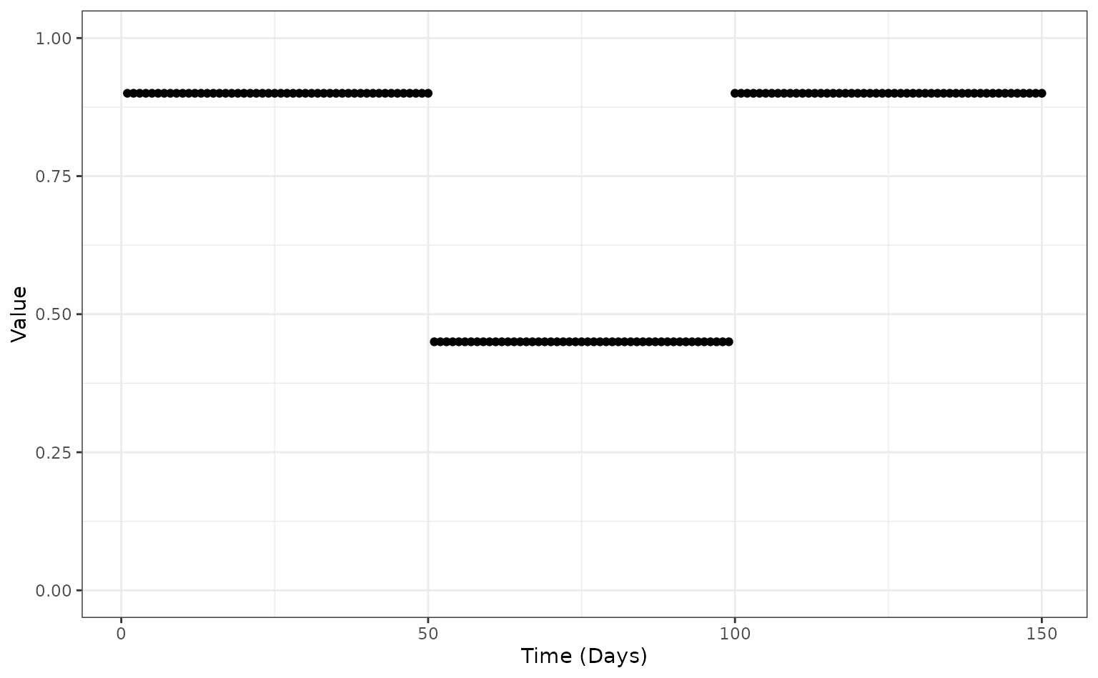

The time-varying case fatality risk function (config$time_varying_death_risk) which scales the hospitalised death risk (hosp_death_risk) and non-hospitalised death risk (non_hosp_death_risk) throughout the epidemic. In this case the risks are at their maximum, user-supplied, values from day 0 to day 50, and then half the risks from day 50 to day 100, and then return to their maximum value from day 100 onwards.

Simulating with the stepwise time-varying case fatality risk:

linelist <- sim_linelist(
  contact_distribution = contact_distribution,
  infectious_period = infectious_period,
  prob_infection = 0.5,
  onset_to_hosp = onset_to_hosp,
  onset_to_death = onset_to_death,
  hosp_death_risk = 0.9,
  non_hosp_death_risk = 0.75,
  outbreak_size = c(500, 1000),
  config = config
)

head(linelist)
#>   id     case_name case_type sex age date_onset date_admission   outcome
#> 1  1  Amoria Goode confirmed   f  40 2023-01-01           <NA>      died
#> 2  3   Niko Aragon confirmed   m   5 2023-01-05           <NA> recovered
#> 3  4 Kirsten Begay confirmed   f  64 2023-01-06           <NA>      died
#> 4  5  Anthony Wang confirmed   m  14 2023-01-07           <NA>      died
#> 5  7      Tim Vang confirmed   m  84 2023-01-09           <NA>      died
#> 6  8 Jordan Bowman confirmed   m  64 2023-01-09           <NA> recovered
#>   date_outcome date_first_contact date_last_contact ct_value
#> 1   2023-01-13               <NA>              <NA>     24.9
#> 2         <NA>         2023-01-03        2023-01-05     24.9
#> 3   2023-02-05         2023-01-02        2023-01-06     24.9
#> 4   2023-02-08         2023-01-03        2023-01-07     24.9
#> 5   2023-02-01         2023-01-10        2023-01-11     24.9
#> 6         <NA>         2023-01-05        2023-01-09     24.9

linelist <- linelist %>%
  pivot_wider(
    names_from = outcome,
    values_from = date_outcome
  ) %>%
  rename(
    date_death = died,
    date_recovery = recovered
  )

daily <- incidence(
  linelist,
  date_index = c(
    onset = "date_onset",
    death = "date_death"
  ),
  interval = "daily"
)
daily <- complete_dates(daily)
plot(daily)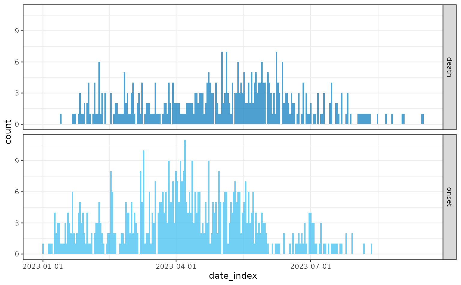

Daily incidence of cases from symptom onset and incidence of deaths. The maximum case fatality risk for hospitalised individuals is 0.9 and for non-hospitalised individuals is 0.75, and these rates remain constant from days 0 to 50, and then from days 50 to 100 the case fatality risk is halved (i.e hosp_death_risk = 0.45 and non_hosp_death_risk = 0.375), before going back to their original risks from day 100 onwards.

This vignette does not explore applying a time-varying case fatality risk to age-stratified fatality risks, but this is possible with the sim_linelist() and sim_outbreak() functions. See the Age-stratified hospitalisation and death risks vignette and combine with instructions from this vignette on setting in a time-varying function using create_config().

The implementation of the time-varying case fatality rate in the simulation functions (sim_linelist() and sim_outbreak()) is flexible to many functional forms. If there are other ways to have a time-varying case fatality risk that are not currently possible please make an issue or pull request. Currently the hospitalisation risk is assumed constant over time can cannot be adjusted to be time-varying like the death risk, if this is a feature you would like included in the {simulist} R package please make the request in an issue.