Estimate individual-level transmission • superspreading

The rate of growth or decline in the incidence of a transmissible infectious disease is often quantified as the population-level reproduction number ( $R$ ). However, there may be individual-level heterogeneity in transmission that this metric does not capture.

In their landmark work, Lloyd-Smith et al. (2005) showed that variation in individual-level disease transmission often exceed that of a poisson model and in some cases that of a geometric model. They fit a negative binomial distribution to show that the distribution of secondary cases displayed overdispersion, in other words, the variance exceeded the mean. In the negative binomial distribution this is quantified by the dispersion ( $k$ ) parameter being less than 1.

This vignette demonstrates how to use the {superspreading} and {fitdistrplus} R packages to estimate the parameters of individual-level transmission and select the best fitting model.

Additionally, {ggplot2} is used for plotting.

library(superspreading)
library(fitdistrplus)
#> Loading required package: MASS
#> Loading required package: survival
library(ggplot2)

Transmission data

For this example we use transmission chain data from Faye et al. (2015) from the Ebola virus disease outbreak in West Africa, between the period from February to August 2014. Specifically, this data reconstructs the pathway of Ebola transmission in Conakry, Guinea.

This data has been used by Althaus (2015) to show that the Ebola outbreak in Conakry displayed signatures of overdispersion (i.e. superspreading events), and by Kucharski et al. (2016) to determine the effectiveness of ring- and mass-vaccination campaigns for ongoing Ebola outbreaks.

# total number of cases (i.e. individuals in transmission chain)
n <- 152

# number of secondary cases for all cases
all_cases_transmission <- c(
  1, 2, 2, 5, 14, 1, 4, 4, 1, 3, 3, 8, 2, 1, 1, 4, 9, 9, 1, 1, 17, 2, 1,
  1, 1, 4, 3, 3, 4, 2, 5, 1, 2, 2, 1, 9, 1, 3, 1, 2, 1, 1, 2
)

# add zeros for each cases that did not cause a secondary case
# (i.e. cases that did not transmit)
all_cases <- c(
  all_cases_transmission,
  rep(0, n - length(all_cases_transmission))
)

# fit a standard set of offspring distribution models:
# - Poisson
# - Geometric
# - Negative Binomial

pois_fit <- fitdist(data = all_cases, distr = "pois")
geom_fit <- fitdist(data = all_cases, distr = "geom")
nbinom_fit <- fitdist(data = all_cases, distr = "nbinom")

model_tbl <- ic_tbl(pois_fit, geom_fit, nbinom_fit)
col.names <- gsub(
  pattern = "^Delta", replacement = "$\\\\Delta$", x = colnames(model_tbl)
)
col.names <- gsub(pattern = "^w", replacement = "$w$", x = col.names)
knitr::kable(model_tbl, col.names = col.names, row.names = FALSE, digits = 1)

distribution	AIC	$\Delta$ AIC	$w$ AIC	BIC	$\Delta$ BIC	$w$ BIC
nbinom	358.4	0.0	1	364.4	0.0	1
geom	413.6	55.2	0	416.6	52.1	0
pois	602.4	244.0	0	605.4	241.0	0

The best performing model, for both AIC and BIC comparison, is the negative binomial.

AIC and BIC are model fitting metrics (information criterion) to determine the model that best fits the data while penalising model complexity to prevent overfitting and allows comparison of models with a different number of parameters. In this case the Poisson and Geometric models have a single parameter, whereas the Negative binomial has two parameters.

nbinom_fit$estimate
#>      size        mu 
#> 0.1814260 0.9537995

The parameter for the negative binomial show that there is overdispersion (size is the dispersion parameter $k$ , and mu is the mean, or $R$ ) in transmission and thus the EVD transmission chain data shows that superspreading events are a possible realisation of EVD transmission dynamics.

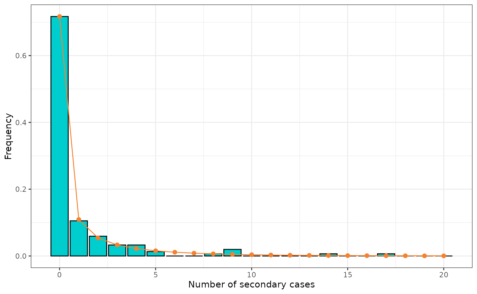
These values match those reported in Althaus (2015) and here we reproduce figure 1 from that paper to display the tail of the distribution from which superspreading events can be possible.

# tally cases
tally <- table(all_cases)

# pad with zeros when number of cases not in tally
num_cases <- rep(0, 21)
names(num_cases) <- as.character(seq(0, 20, 1))
num_cases[names(tally)] <- tally

# convert cases to proportional of total cases to plot on the same scale as
# the density
prop_num_cases <- num_cases / sum(num_cases)

# create data frame with proportion of cases, density and number of secondary
# cases
nbinom_data <- data.frame(
  x = seq(0, 20, 1),
  prop_num_cases = prop_num_cases,
  density = dnbinom(
    x = seq(0, 20, 1),
    size = nbinom_fit$estimate[["size"]],
    mu = nbinom_fit$estimate[["mu"]]
  )
)

# make plot
ggplot(data = nbinom_data) +
  geom_col(
    mapping = aes(x = x, y = prop_num_cases),
    fill = "cyan3",
    colour = "black"
  ) +
  geom_point(
    mapping = aes(x = x, y = density),
    colour = "#f58231",
    size = 2
  ) +
  geom_line(
    mapping = aes(x = x, y = density),
    colour = "#f58231"
  ) +
  scale_x_continuous(name = "Number of secondary cases") +
  scale_y_continuous(name = "Frequency") +
  theme_bw()

Number of secondary cases from the empirical data (bar plot) and the density of the negative binomial with the maximum likelihood estimates when fit to the empirical data (points and line). This plot is reproduced from Althaus (2015) figure 1.

Next we partitioned the data into index cases and secondary cases following Kucharski et al. (2016).

index_case_transmission <- c(2, 17, 5, 1, 8, 2, 14)
secondary_case_transmission <- c(
  1, 2, 1, 4, 4, 1, 3, 3, 1, 1, 4, 9, 9, 1, 2, 1, 1, 1, 4, 3, 3, 4, 2,
  5, 1, 2, 2, 1, 9, 1, 3, 1, 2, 1, 1, 2
)

# Format data into index and non-index cases

# total non-index cases
n_non_index <- sum(c(index_case_transmission, secondary_case_transmission))
# transmission from all non-index cases
non_index_cases <- c(
  secondary_case_transmission,
  rep(0, n_non_index - length(secondary_case_transmission))
)

We fit the negative binomial model for both the index and non-index case transmission events.

# Estimate R and k for index and non-index cases
param_index <- fitdist(
  data = index_case_transmission,
  distr = "nbinom"
)
param_index
#> Fitting of the distribution ' nbinom ' by maximum likelihood 
#> Parameters:
#>      estimate Std. Error
#> size 1.596646   1.025029
#> mu   7.000771   2.320850
param_non_index <- fitdist(
  data = non_index_cases,
  distr = "nbinom"
)
param_non_index
#> Fitting of the distribution ' nbinom ' by maximum likelihood 
#> Parameters:
#>       estimate Std. Error
#> size 0.1937490 0.05005421
#> mu   0.6619608 0.14197451

Superspreading using alternative distributions

Advanced options

This section of the vignette discusses some alternative transmission models to quantify overdispersion and may be considered advanced in comparison to the above example.

Research subsequent to Lloyd-Smith et al. (2005) has shown that contact data from infectious disease outbreaks often shows signatures of overdispersion and can therefore cause superspreading events. However, overdispersion can be modelled by other distributions to the negative binomial.

Kremer et al. (2021) showed for SARS-CoV-2 that superspreading may be better modelled by a Poisson mixture distribution (or Poisson compound distribution). Four Poisson mixture distribution were applied: Poisson-Gamma, Poisson-Lognormal, Poisson-Weibull, and Poisson-Generalised-Gamma; finding the Poisson-lognormal and Poisson-Weibull fit best for three data sets.

The Poisson-Gamma distribution is the same as the negative binomial distribution. Hereafter we refer to it is the negative binomial.

R has the density functions and cumulative distribution functions for the poisson (dpois() and ppois()), geometric (dgeom() and pgeom()) and negative binomial (dnbinom() and pnbinom()) distributions, but does not supply Poisson compound distributions.

In the {superspreading} R package we supply the density and cumulative distribution functions for the Poisson-lognormal (dpoislnorm() and ppoislnorm()) and Poisson-Weibull (dpoisweibull() and ppoisweibull()).

These functions can be used with {fitdistrplus}, as shown for the other distributions above.

# fit an expanded set of offspring distribution models:
# - Poisson
# - Geometric
# - Negative Binomial
# - Poisson-lognormal compound
# - Poisson-Weibull compound

pois_fit <- fitdist(data = all_cases, distr = "pois")
geom_fit <- fitdist(data = all_cases, distr = "geom")
nbinom_fit <- fitdist(data = all_cases, distr = "nbinom")
poislnorm_fit <- fitdist(
  data = all_cases,
  distr = "poislnorm",
  start = list(meanlog = 1, sdlog = 1)
)
poisweibull_fit <- fitdist(
  data = all_cases,
  distr = "poisweibull",
  start = list(shape = 1, scale = 1)
)

model_tbl <- ic_tbl(
  pois_fit, geom_fit, nbinom_fit, poislnorm_fit, poisweibull_fit
)
col.names <- gsub(
  pattern = "^Delta", replacement = "$\\\\Delta$", x = colnames(model_tbl)
)
col.names <- gsub(pattern = "^w", replacement = "$w$", x = col.names)
knitr::kable(model_tbl, col.names = col.names, row.names = FALSE, digits = 1)

distribution	AIC	$\Delta$ AIC	$w$ AIC	BIC	$\Delta$ BIC	$w$ BIC
nbinom	358.4	0.0	0.6	364.4	0.0	0.6
poisweibull	359.8	1.4	0.3	365.9	1.4	0.3
poislnorm	362.8	4.4	0.1	368.9	4.4	0.1
geom	413.6	55.2	0.0	416.6	52.1	0.0
pois	602.4	244.0	0.0	605.4	241.0	0.0

The negative binomial is still the best performing fitting model, even with the addition of the Poisson-lognormal and Poisson-Weibull models. Although the second best model, the Poisson-Weibull, performs similarly well to the negative binomial ( $\Delta$ AIC < 2 & $\Delta$ BIC < 2).

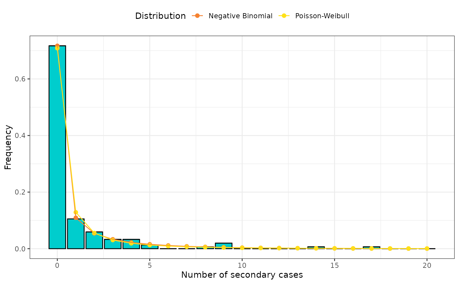
Here we plot the density of each distribution given the maximum likelihood estimates to inspect differences between the two distributions.

# create data frame with proportion of cases, density of each distribution
dist_compare_data <- data.frame(
  x = seq(0, 20, 1),
  prop_num_cases = c(prop_num_cases, rep(0, 21)),
  dens = c(
    dnbinom(
      x = seq(0, 20, 1),
      size = nbinom_fit$estimate[["size"]],
      mu = nbinom_fit$estimate[["mu"]]
    ),
    poisweibull_density = dpoisweibull(
      x = seq(0, 20, 1),
      shape = poisweibull_fit$estimate[["shape"]],
      scale = poisweibull_fit$estimate[["scale"]]
    )
  ),
  dist = c(rep("Negative Binomial", 21), rep("Poisson-Weibull", 21))
)

# make plot
ggplot(data = dist_compare_data) +
  geom_col(
    mapping = aes(x = x, y = prop_num_cases),
    fill = "cyan3",
    colour = "black"
  ) +
  geom_point(
    mapping = aes(
      x = x,
      y = dens,
      colour = dist
    ),
    size = 2
  ) +
  geom_line(mapping = aes(x = x, y = dens, colour = dist)) +
  scale_x_continuous(name = "Number of secondary cases") +
  scale_y_continuous(name = "Frequency") +
  scale_colour_manual(
    name = "Distribution",
    values = c("#f58231", "#ffe119")
  ) +
  theme_bw() +
  theme(legend.position = "top")

Number of secondary cases from the empirical data (bar plot) and the density of the negative binomial (orange) and poisson-Weibull (pink) with the maximum likelihood estimates when fit to the empirical data (points and line).

The fit of each model is very similar, as expected from the close AIC and BIC (these models have the same numbers of free parameters). The Poisson-Weibull compound distribution can adequately capture the overdispersion in the EVD transmission data. A noticeable difference between the models fitting to the number of cases that caused a single secondary cases. Here the negative binomial matches the empirical data, whereas the Poisson-Weibull slightly overestimates the number.

Overall, {superspreading} and {fitdistrplus} (or another fitting package of your choice) can be used to estimate and understand individual-level transmission dynamics when transmission chain data is available.

References

Althaus, Christian L. 2015. “Ebola Superspreading.” The Lancet Infectious Diseases 15 (5): 507–8. https://doi.org/10.1016/S1473-3099(15)70135-0.

Faye, Ousmane, Pierre-Yves Boëlle, Emmanuel Heleze, Oumar Faye, Cheikh Loucoubar, N’Faly Magassouba, Barré Soropogui, et al. 2015. “Chains of Transmission and Control of Ebola Virus Disease in Conakry, Guinea, in 2014: An Observational Study.” The Lancet Infectious Diseases 15 (3): 320–26. https://doi.org/10.1016/S1473-3099(14)71075-8.

Kremer, Cécile, Andrea Torneri, Sien Boesmans, Hanne Meuwissen, Selina Verdonschot, Koen Vanden Driessche, Christian L. Althaus, Christel Faes, and Niel Hens. 2021. “Quantifying Superspreading for COVID-19 Using Poisson Mixture Distributions.” Scientific Reports 11 (1): 14107. https://doi.org/10.1038/s41598-021-93578-x.

Kucharski, Adam J., Rosalind M. Eggo, Conall H. Watson, Anton Camacho, Sebastian Funk, and W. John Edmunds. 2016. “Effectiveness of Ring Vaccination as Control Strategy for Ebola Virus Disease.” Emerging Infectious Diseases 22 (1): 105–8. https://doi.org/10.3201/eid2201.151410.

Lloyd-Smith, J. O., S. J. Schreiber, P. E. Kopp, and W. M. Getz. 2005. “Superspreading and the Effect of Individual Variation on Disease Emergence.” Nature 438 (7066): 355–59. https://doi.org/10.1038/nature04153.