Outbreaks in heterogeneous networks • superspreading

library(superspreading)
library(ggplot2)
library(scales)

Determining if an outbreak will grow and spread through a susceptible population is quantified by the basic reproduction number ( $R_0$ ). When there is individual-level variability in the connectedness of different individuals in a network (i.e. higher variance in the degree of each node) it can lead to heterogeneity in transmission dynamics. Such scenarios are common in persistent sexually transmitted infections (STIs), where partners can change during the infectious period, which means highly connected individuals can be both more likely to acquire and pass on the infection.

Under the basic assumption of homogeneous contact patterns (i.e. no network effects), we have the following expression for the basic reproduction number:

$R_0 = \frac{\beta M}{\gamma}$ where $\beta$ is the probability of transmission per contact, $1/\gamma$ is the duration of infectiousness ( $\gamma$ is the rate of loss of infectiousness) and $M$ is the mean number of contacts (or partners) per unit time (e.g., per year).

In contrast, May and Anderson (1988) showed that the transmissibility of an infectious disease in a heterogeneous network can be defined as follows:

$R_0 = \frac{\beta}{\gamma} \frac{M^2 + V}{M}$ where $V$ is the variance of the number of contacts per unit time. This formulation can be appropriate if heterogeneity is predictable over time (i.e. highly connected individuals typically remain highly connected), the duration of infectiousness is similar or longer to the frequency of partner change among highly connected individuals, and the disease has the potential to cause a substantial outbreak (i.e. larger value of $\beta$ and/or $1/\gamma$ ).

The {superspreading} package provides the calc_network_R() function to calculate the reproduction number using the unadjusted formula (first equation) and the adjusted formula (second equation).

For example, the possibility of a sexually transmitted Zika virus outbreak was a particular concern when the infection spread globally in 2015-16. Yakob et al. (2016) used the above heterogeneous network model to determine the risk that sexual transmission could be a common mode of transmission for Zika virus, leading to sustained human-to-human transmission in the absence of vectors.

Here we replicate the analysis of Yakob et al. (2016) to show the low likelihood of Zika causing an outbreak from sexual transmission. Following Yakob et al. (2016), we use data from the National Survey of Sexual Attitude and Lifestyles (Natsal) on the mean and variance in the number of sexual partners and age range (Mercer et al. 2013).

infect_duration <- exp(seq(log(0.01), log(10), length.out = 100))
prob_transmission <- exp(seq(log(0.01), log(1), length.out = 100))
params <- expand.grid(
  infect_duration = infect_duration,
  prob_transmission = prob_transmission
)
R <- t(apply(
  params,
  MARGIN = 1,
  function(x) {
    calc_network_R(
      mean_num_contact = 14.1,
      sd_num_contact = 69.6,
      infect_duration = x[["infect_duration"]],
      prob_transmission = x[["prob_transmission"]],
      age_range = c(16, 74)
    )
  }
))
res <- cbind(params, R)
res <- reshape(
  data = res,
  varying = c("R", "R_net"),
  v.names = "R",
  direction = "long",
  times = c("R", "R_net"),
  timevar = "group"
)

ggplot(data = res) +
  geom_tile(
    mapping = aes(
      x = infect_duration,
      y = prob_transmission,
      fill = R
    )
  ) +
  geom_contour(
    mapping = aes(
      x = infect_duration,
      y = prob_transmission,
      z = R
    ),
    breaks = 1,  # Set the contour line at R = 1
    colour = "black"
  ) +
  scale_x_continuous(
    name = "Mean duration of infectiousness",
    trans = "log", breaks = breaks_log()
  ) +
  scale_y_continuous(
    name = "Zika virus transmission probability per sexual partners",
    trans = "log", breaks = breaks_log()
  ) +
  facet_wrap(
    vars(group),
    labeller = as_labeller(c(R = "R", R_net = "Adjusted R"))
  ) +
  scale_fill_viridis_c(
    trans = "log",
    breaks = breaks_log(n = 8)(min(res$R):max(res$R)),
    labels = label_comma()
  ) +
  theme_bw()

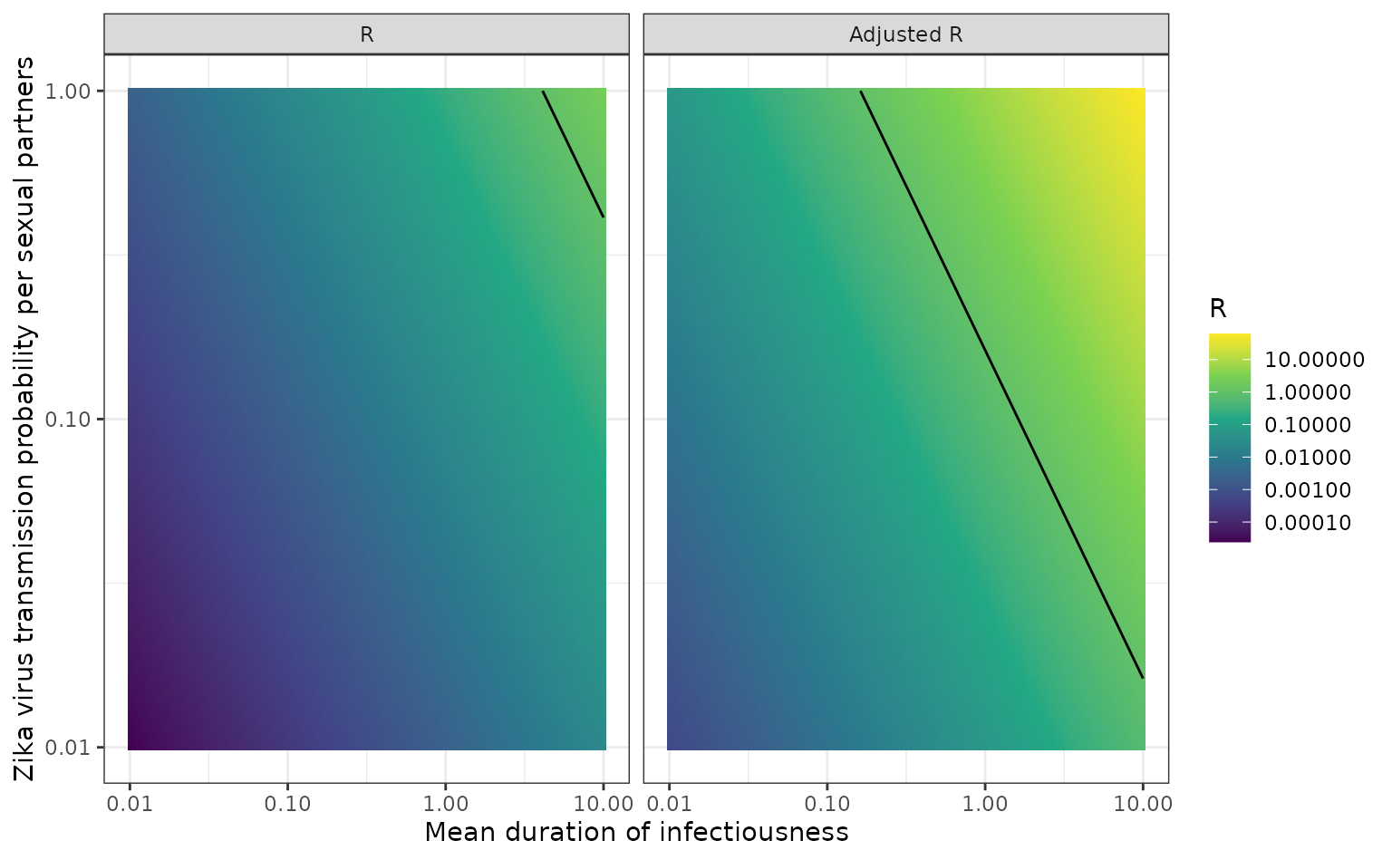
The reproduction number using the unadjusted and adjusted calculation – calculated using calc_network_R() – with mean duration of infection on the x-axis and transmission probability per sexual partner on the y-axis. The line shows the points that $R_0$ is equal to one. Both axes are plotted on a natural log scale. This plot is similar to Figure 1 from Yakob et al. (2016), but is plotted as a heatmap and without annotation.

Another study that showed the network effects on transmission of an STI was Endo et al. (2022), who estimated that Mpox (or monkeypox) could spread throughout a network on men who have sex with men (MSM), but would have lower transmissibility in the wider population. Using the Natsal UK data (Mercer et al. 2013) on same- and opposite-sex sexual partnerships for the age range of 18 to 44, they show that the disease transmission for MSM is greater than for a non-MSM transmission network. Because Mpox has a relatively short infectious period, this study assumed that contacts remained fixed during the period of infection, and hence used a next generation matrix approach more akin to the group-specific transmission defined in the finalsize package.

For comparison, we produce a figure similar to Endo et al. (2022), using calc_network_R() instead to show how highly connected individuals – who are more likely to acquire and pass on infection – alter the estimated $R_0$ compared to the simpler assumption of $R_0 = SAR \times contacts$ , under the assumptions described above.

beta <- seq(0.001, 1, length.out = 1000)
duration_years <- 21 / 365
res <- lapply(
  beta,
  calc_network_R,
  mean_num_contact = 10,
  sd_num_contact = 50,
  infect_duration = duration_years,
  age_range = c(18, 44)
)
res <- do.call(rbind, res)
res <- as.data.frame(cbind(beta, res))
res <- reshape(
  data = res,
  varying = c("R", "R_net"),
  v.names = "R",
  direction = "long",
  times = c("R", "R_net"),
  timevar = "group"
)

ggplot(data = res) +
  geom_line(mapping = aes(x = beta, y = R, colour = group)) +
  geom_hline(mapping = aes(yintercept = 1)) +
  scale_y_continuous(
    name = "Reproduction Number (R)",
    trans = "log",
    breaks = breaks_log(),
    labels = label_comma()
  ) +
  scale_x_continuous(name = "Secondary Attack Rate (SAR)") +
  scale_colour_brewer(
    name = "Reproduction Number",
    labels = c("R", "Adjusted R"),
    palette = "Set1"
  ) +
  theme_bw() +
  theme(legend.position = "top")

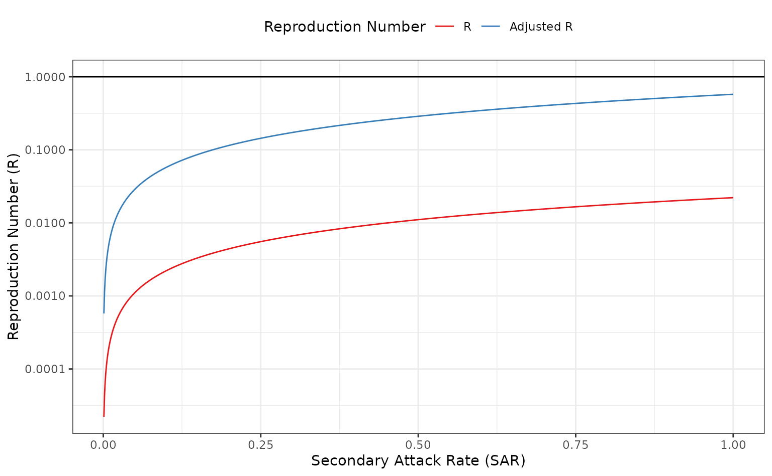
The reproduction number using the unadjusted and adjusted calculation – calculated using calc_network_R() – with secondary attack rate on the x-axis and reproduction number ( $R_0$ ) on the y-axis. This plot is similar to Figure 2A from Endo et al. (2022).

Methodological caveat: There is a link with the theory for the main negative binomial models from the superspreading package here (which have a Gamma distributed mean), because the above Anderson and May formulation requires the ‘true’ mean and variance of the underlying static contact distribution, rather than the observed mean and variance. To give the superspreading version: in a simple branching process with fixed $R_0$ (i.e. zero variance in the individual-level reproduction number, perhaps because everyone has an identical number of contacts), the Poisson distributed number of transmissions per year measured exhibits more variation than the ‘true’ $R_0$ (which has zero variance). For the above STI model, taking the lifetime average deals with this problem some extent, because if we look at the sum of contacts over a large number of years, then calculate the mean per year, the observed distribution will converge as the number of years gets very large.

References

Endo, Akira, Hiroaki Murayama, Sam Abbott, Ruwan Ratnayake, Carl A. B. Pearson, W. John Edmunds, Elizabeth Fearon, and Sebastian Funk. 2022. “Heavy-Tailed Sexual Contact Networks and Monkeypox Epidemiology in the Global Outbreak, 2022.” Science 378 (6615): 90–94. https://doi.org/10.1126/science.add4507.

May, Robert, and Roy Anderson. 1988. “The Transmission Dynamics of Human Immunodeficiency Virus (HIV).” Philosophical Transactions of the Royal Society of London. B, Biological Sciences 321 (1207): 565–607. https://doi.org/10.1098/rstb.1988.0108.

Mercer, Catherine H, Clare Tanton, Philip Prah, Bob Erens, Pam Sonnenberg, Soazig Clifton, Wendy Macdowall, et al. 2013. “Changes in Sexual Attitudes and Lifestyles in Britain Through the Life Course and over Time: Findings from the National Surveys of Sexual Attitudes and Lifestyles (Natsal).” The Lancet 382 (9907): 1781–94. https://doi.org/10.1016/S0140-6736(13)62035-8.

Yakob, Laith, Adam Kucharski, Stephane Hue, and W John Edmunds. 2016. “Low Risk of a Sexually-Transmitted Zika Virus Outbreak.” The Lancet Infectious Diseases 16 (10): 1100–1102. https://doi.org/10.1016/S1473-3099(16)30324-3.