Create a short-term forecast
Last updated on 2024-09-24 | Edit this page
Overview
Questions
- How do I create short-term forecasts from case data?
- How do I account for incomplete reporting in forecasts?
Objectives
- Learn how to make forecasts of cases using R package
EpiNow2 - Learn how to include an observation process in estimation
Prerequisites
- Complete tutorial Quantifying transmission
Learners should familiarise themselves with following concept dependencies before working through this tutorial:
Statistics : probability distributions, principle of Bayesian analysis.
Epidemic theory : Effective reproduction number.
Introduction
Given case data, we can create estimates of the current and future number of cases by accounting for both delays in reporting and under reporting. To make statements about the future, we need to make an assumption of how observations up to today are related to what we expect to happen in the future. The simplest way of doing so is to assume “no change”, i.e. the reproduction number remains the same in the future as last observed. In this tutorial we will create short-term forecasts by assuming the reproduction number will remain the same as it was estimated to be on the final date for which data was available.
Create a short-term forecast
The function epinow() described in the previous tutorial
is a wrapper for the function estimate_infections() used to
estimate cases by date of infection. Using the same code in the previous
tutorial we can extract the short-term forecast using:
R
reported_cases <- cases[1:90, ]
estimates <- epinow(
  reported_cases = reported_cases,
  generation_time = generation_time_opts(generation_time_fixed),
  delays = delay_opts(incubation_period_fixed + reporting_delay_fixed),
  rt = rt_opts(prior = list(mean = rt_log_mean, sd = rt_log_sd))
)
OUTPUT
WARN [2024-09-24 02:14:50] epinow: There were 6 divergent transitions after warmup. See
https://mc-stan.org/misc/warnings.html#divergent-transitions-after-warmup
to find out why this is a problem and how to eliminate them. -
WARN [2024-09-24 02:14:50] epinow: Examine the pairs() plot to diagnose sampling problems
-
WARN [2024-09-24 02:14:52] epinow: Bulk Effective Samples Size (ESS) is too low, indicating posterior means and medians may be unreliable.
Running the chains for more iterations may help. See
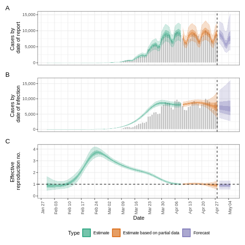
https://mc-stan.org/misc/warnings.html#bulk-ess - We can visualise the estimates of the effective reproduction number
and the estimated number of cases using plot(). The
estimates are split into three categories:
Estimate (green): utilises all data,
Estimate based on partial data (orange): estimates that are based less data are therefore more uncertain,
Forecast (purple): forecasts into the future.
R
plot(estimates)
Forecasting with estimates of \(R_t\)
By default, the short-term forecasts are created using the latest estimate of the reproduction number \(R_t\). As this estimate is based on partial data, it has considerable uncertainty.
The reproduction number that is projected into the future can be
changed to a less recent estimate based on more data using
rt_opts():
R
rt_opts(future = "estimate")
The result will be less uncertain forecasts (as they are based on \(R_t\) with a narrower uncertainty interval) but the forecasts will be based on less recent estimates of \(R_t\) and assume no change since then.
Additionally, there is the option to project the value of \(R_t\) into the future using a generic model
by setting future = "project". As this option uses a model
to forecast the value of \(R_t\), the
result will be forecasts that are more uncertain than
estimate, for an example see
here.
Incomplete observations
In the previous tutorial we accounted for delays in reporting. In
EpiNow2 we also can account for incomplete observations as
in reality, 100% of cases are not reported.
We will pass another input into epinow() called
obs to define an observation model. The format of
obs must be the obs_opt() function (see
?EpiNow2::obs_opts for more detail).
Let’s say we believe the COVID-19 outbreak data from the previous
tutorial do not include all reported cases. We believe that we only
observe 40% of cases. To specify this in the observation model, we must
pass a scaling factor with a mean and standard deviation. If we assume
that 40% of cases are in the case data (with standard deviation 1%),
then we specify the scale input to obs_opts()
as follows:
R
obs_scale <- list(mean = 0.4, sd = 0.01)
To run the inference framework with this observation process, we add
obs = obs_opts(scale = obs_scale) to the input arguments of
epinow():
R
obs_scale <- list(mean = 0.4, sd = 0.01)
reported_cases <- cases[1:90, ]
estimates <- epinow(
  reported_cases = reported_cases,
  generation_time = generation_time_opts(generation_time_fixed),
  delays = delay_opts(incubation_period_fixed + reporting_delay_fixed),
  rt = rt_opts(prior = list(mean = rt_log_mean, sd = rt_log_sd)),
  obs = obs_opts(scale = obs_scale)
)
OUTPUT
WARN [2024-09-24 02:21:47] epinow: There were 4 divergent transitions after warmup. See
https://mc-stan.org/misc/warnings.html#divergent-transitions-after-warmup
to find out why this is a problem and how to eliminate them. -
WARN [2024-09-24 02:21:47] epinow: Examine the pairs() plot to diagnose sampling problems
 -
R
summary(estimates)
OUTPUT
                                 measure                 estimate
                                  <char>                   <char>
1: New confirmed cases by infection date   18060 (10134 -- 32193)
2:        Expected change in daily cases        Likely decreasing
3:            Effective reproduction no.        0.9 (0.57 -- 1.3)
4:                        Rate of growth -0.014 (-0.065 -- 0.039)
5:          Doubling/halving time (days)          -51 (18 -- -11)
The estimates of transmission measures such as the effective reproduction number and rate of growth are similar (or the same in value) compared to when we didn’t account for incomplete observations (see previous tutorial). However the number of new confirmed cases by infection date has changed substantially in magnitude to reflect the assumption that only 40% of cases are in the data set.
We can also change the default distribution from Negative Binomial to
Poisson, remove the default week effect and more. See
?EpiNow2::obs_opts for more detail.
Forecast secondary observations
EpiNow2 also has the ability to estimate and forecast
secondary observations e.g. deaths, hospitalisations from a primary
observation e.g. cases. Here we will illustrate how to forecast the
number of deaths arising from observed cases of COVID-19 in the early
stages of the UK outbreak.
First, we must format our data to have the following columns:
-
date: the date (as a date object see?is.Date()), -
primary: number of primary observations on that date, in this example cases, -
secondary: number of secondary observations date, in this example deaths.
R
reported_cases_deaths <- aggregate(
  cbind(cases_new, deaths_new) ~ date,
  data =
    incidence2::covidregionaldataUK[, c("date", "cases_new", "deaths_new")],
  FUN = sum
)
colnames(reported_cases_deaths) <- c("date", "primary", "secondary")
Using the first 30 days of data on cases and deaths, we will estimate
the relationship between the primary and secondary observations using
estimate_secondary(), then forecast future deaths using
forecast_secondary(). For detail on the model see the model
documentation.
We must specify the type of observation using type in
secondary_opts(), options include:
- “incidence” : secondary observations arise from previous primary observations, i.e. deaths arising from recorded cases.
- “prevalence” : secondary observations arise from a combination current primary observations and past secondary observations, i.e. hospital bed usage arising from current hospital admissions and past hospital bed usage.
In this example we specify
secondary_opts(type = "incidence"). See
?EpiNow2::secondary_opts for more detail).
The final key input is the delay distribution between the primary and
secondary observations. Here this is the delay between case report and
death, we assume this follows a gamma distribution with mean of 14 days
and standard deviation of 5 days. Using dist_spec() we
specify a fixed gamma distribution.
There are further function inputs to
estimate_secondary() which can be specified, including
adding an observation process, see
?EpiNow2::estimate_secondary for detail on the options.
To find the model fit between cases and deaths :
R
estimate_cases_to_deaths <- estimate_secondary(
  reports = reported_cases_deaths[1:30, ],
  secondary = secondary_opts(type = "incidence"),
  delays = delay_opts(dist_spec(
    mean = 14, sd = 5,
    max = 30, distribution = "gamma"
  ))
)
Be cautious of timescale
In the early stages of an outbreak there can be substantial changes in testing and reporting. If there are testing changes from one month to another, then there will be a bias in the model fit. Therefore, you should be cautious of the time-scale of data used in the model fit and forecast.
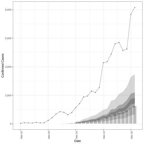
We plot the model fit (shaded ribbons) with the secondary observations (bar plot) and primary observations (dotted line) as follows:
R
plot(estimate_cases_to_deaths, primary = TRUE)
To use this model fit to forecast deaths, we pass a data frame consisting of the primary observation (cases) for dates not used in the model fit.
Note : in this tutorial we are using data where we know the deaths and cases, so we create a data frame by extracting the cases. But in practice, this would be a different data set consisting of cases only.
R
cases_to_forecast <- reported_cases_deaths[31:60, c("date", "primary")]
colnames(cases_to_forecast) <- c("date", "value")
To forecast, we use the model fit
estimate_cases_to_deaths:
R
deaths_forecast <- forecast_secondary(
  estimate = estimate_cases_to_deaths,
  primary = cases_to_forecast
)
plot(deaths_forecast)
WARNING
Warning: Removed 30 rows containing missing values (`position_stack()`).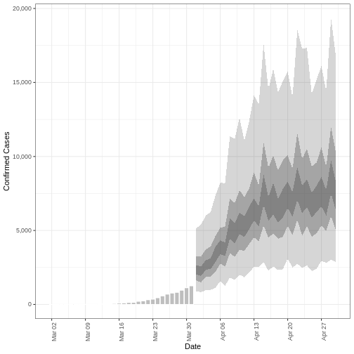
The plot shows the forecast secondary observations (deaths) over the
dates which we have recorded cases for. It is also possible to forecast
deaths using forecast cases, here you would specify primary
as the estimates output from
estimate_infections().
Challenge : Ebola outbreak analysis
Challenge
Download the file ebola_cases.csv and read it into R. The simulated data consists of the date of symptom onset and number of confirmed cases of the early stages of the Ebola outbreak in Sierra Leone in 2014.
Using the first 3 months (120 days) of data:
- Estimate of cases increasing or decreasing on day 120 of the outbreak (Hint: Find the effective reproduction number and growth rate on day 120)
- Create a two week forecast of number of cases
You can use the following parameter values for the delay distribution(s) and generation time distribution.
- Incubation period : Log normal\((2.487,0.330)\) (Eichner et
al. 2011 via
{epiparameter}) - Generation time : Gamma\((15.3, 10.1)\) (WHO Ebola Response Team 2014)
You may include some uncertainty around the mean and standard deviation of these distributions.
Ensure the data is in the correct format :
-
date: the date (as a date object see?is.Date()), -
confirm: number of confirmed cases on that date.
To estimate the effective reproduction number and growth rate, we
will use the function epinow().
As the data consists of date of symptom onset, we only need to specify a delay distribution for the incubation period and the generation time.
We specify the distributions with some uncertainty around the mean and standard deviation of the log normal distribution for the incubation period and the Gamma distribution for the generation time.
R
ebola_incubation_period <- dist_spec(
  mean = 2.487, sd = 0.330,
  mean_sd = 0.5, sd_sd = 0.5,
  max = 20, distribution = "lognormal"
)

ebola_generation_time <- dist_spec(
  mean = 15.3, sd = 10.1,
  mean_sd = 0.5, sd_sd = 0.5,
  max = 30, distribution = "gamma"
)
As we want to also create a two week forecast, we specify
horizon = 14 to forecast 14 days instead of the default 7
days.
R
# read data
# e.g.: if path to file is data/raw-data/ebola_cases.csv then:
ebola_cases <-
  read.csv(here::here("data", "raw-data", "ebola_cases.csv"))
R
# format date column
ebola_cases$date <- as.Date(ebola_cases$date)

ebola_estimates <- epinow(
  reported_cases = ebola_cases[1:120, ], # first 3 months of data only
  generation_time = generation_time_opts(ebola_generation_time),
  delays = delay_opts(ebola_incubation_period),
  # horizon needs to be 14 days to create two week forecast (default is 7 days)
  horizon = 14
)
OUTPUT
WARN [2024-09-24 02:23:54] epinow: There were 24 divergent transitions after warmup. See
https://mc-stan.org/misc/warnings.html#divergent-transitions-after-warmup
to find out why this is a problem and how to eliminate them. -
WARN [2024-09-24 02:23:54] epinow: Examine the pairs() plot to diagnose sampling problems
 -
R
summary(ebola_estimates)
OUTPUT
                                 measure                estimate
                                  <char>                  <char>
1: New confirmed cases by infection date         102 (47 -- 265)
2:        Expected change in daily cases              Increasing
3:            Effective reproduction no.        1.7 (1.1 -- 2.9)
4:                        Rate of growth 0.043 (0.0041 -- 0.091)
5:          Doubling/halving time (days)         16 (7.6 -- 170)
The effective reproduction number \(R_t\) estimate (on the last date of the data) is 1.7 (1.1 – 2.9). The exponential growth rate of case numbers is 0.043 (0.0041 – 0.091).
Visualize the estimates:
R
plot(ebola_estimates)
Summary
EpiNow2 can be used to create short term forecasts and
to estimate the relationship between different outcomes. There are a
range of model options that can be implemented for different analysis,
including adding an observational process to account for incomplete
reporting. See the vignette
for more details on different model options in EpiNow2 that
aren’t covered in these tutorials.
Key Points
- We can create short-term forecasts by making assumptions about the future behaviour of the reproduction number
- Incomplete case reporting can be accounted for in estimates