Read delays
Last updated on 2024-09-24 | Edit this page
Overview
Questions
- How to get delay distributions from a systematic review?
- How to connect reused delays with my existing analysis pipeline?
- When should delays be reused from a systematic review?
Objectives
- Get delays from a systematic review with
{epiparameter}. - Get statistical summaries and distribution parameters of delay distributions.
- Use distribution functions from delay distributions.
- Convert a continuous to a discrete delay distribution.
Prerequisites
This episode requires you to be familiar with:
Data science : Basic programming with R.
Epidemic theory : Epidemiological parameters. Time periods.
Introduction
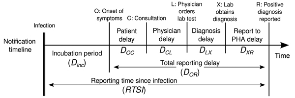
The natural history of an infectious disease shows that its development has a regularity from stage to stage. The time periods from an infectious disease inform about the timing of transmission and interventions.
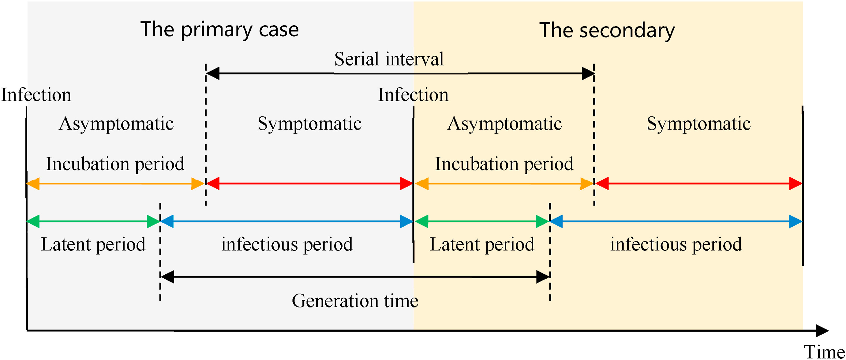
Definitions
Look at the glossary for the definitions of all the time periods of the figure above!
However, early in an epidemic, modelling efforts can be delayed by
the lack of a centralized resource that summarises input parameters for
the disease of interest (Nash et al., 2023).
Projects like {epiparameter} and {epireview}
are building online catalogues following systematic review protocols
that can help build models faster for coming outbreaks and epidemics
from known pathogens and unknown ones related to known families of
viruses.
To exemplify how to use {epiparameter} in your analysis
pipeline, our goal in this episode will be to replace the
generation_time input that we can use for
EpiNow2::epinow().
R
epinow_estimates <- epinow(
  # cases
  reported_cases = example_confirmed[1:60],
  # delays
  generation_time = generation_time_opts(generation_time),
  # computation
  stan = stan_opts(
    cores = 4, samples = 1000, chains = 3,
    control = list(adapt_delta = 0.99)
  )
)
To do this replacement, instead of plug-in numeric values to
EpiNow2::dist_spec() to manually specify the delay
distribution parameters, we are going to collect them from the library
of epidemiological parameters provided by
{epiparameter}:
R
generation_time <- dist_spec(
  mean = 3.6,
  sd = 3.1,
  max = 20,
  distribution = "lognormal"
)
Let’s explore how we can access this and other time delays using
{epiparameter}. We’ll use the pipe %>% to
connect some of their functions, so let’s also call to the
tidyverse package:
R
library(epiparameter)
library(EpiNow2)
library(tidyverse)
Find a Generation time
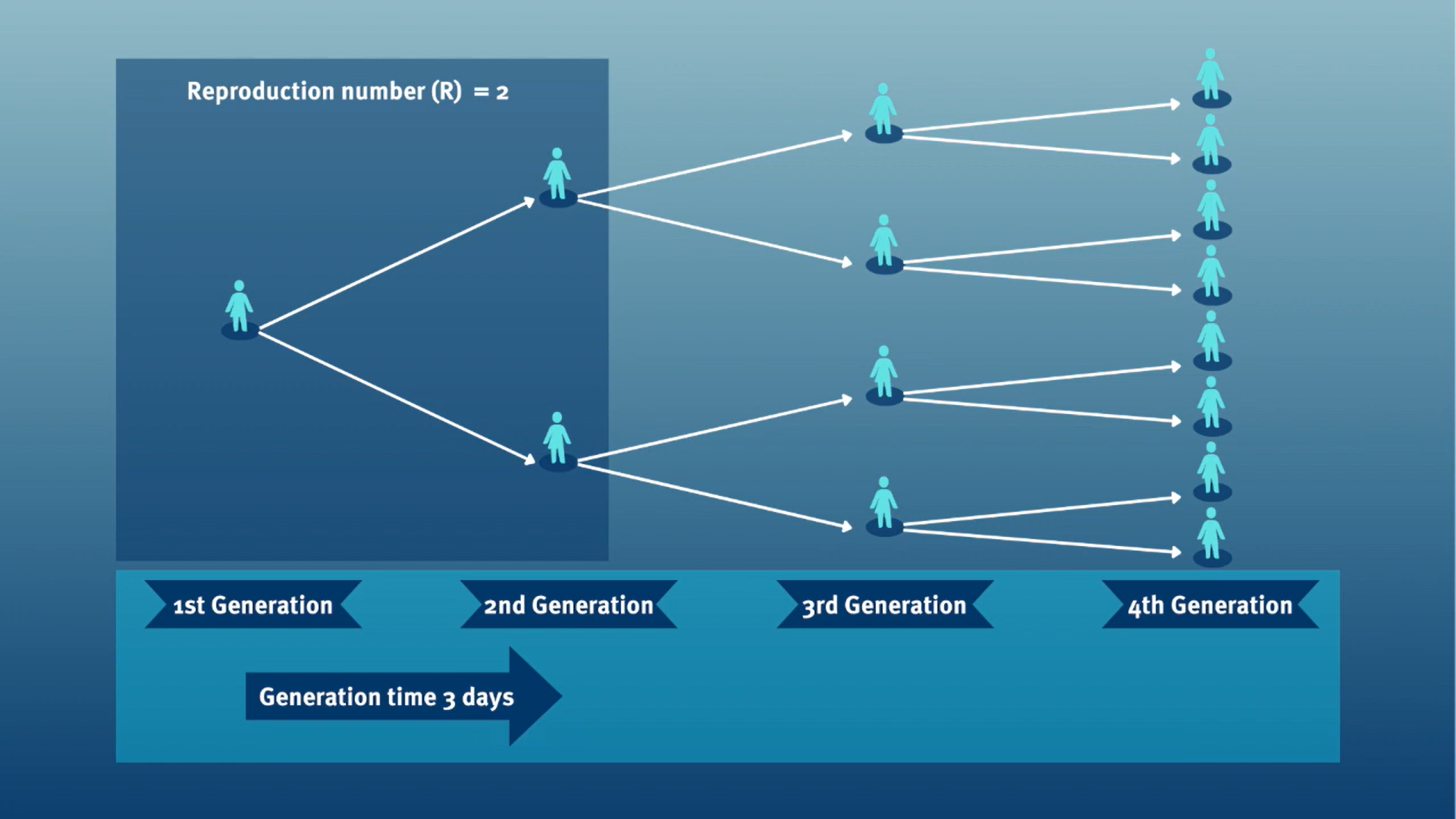
The generation time, jointly with the \(R\), can inform about the speed of spread and its feasibility of control. Given a \(R>1\), with a shorter generation time, cases can appear more quickly.
In calculating the effective reproduction number (\(R_{t}\)), the generation time distribution is often approximated by the serial interval distribution. This frequent approximation is because it is easier to observe and measure the onset of symptoms than the onset of infectiousness.
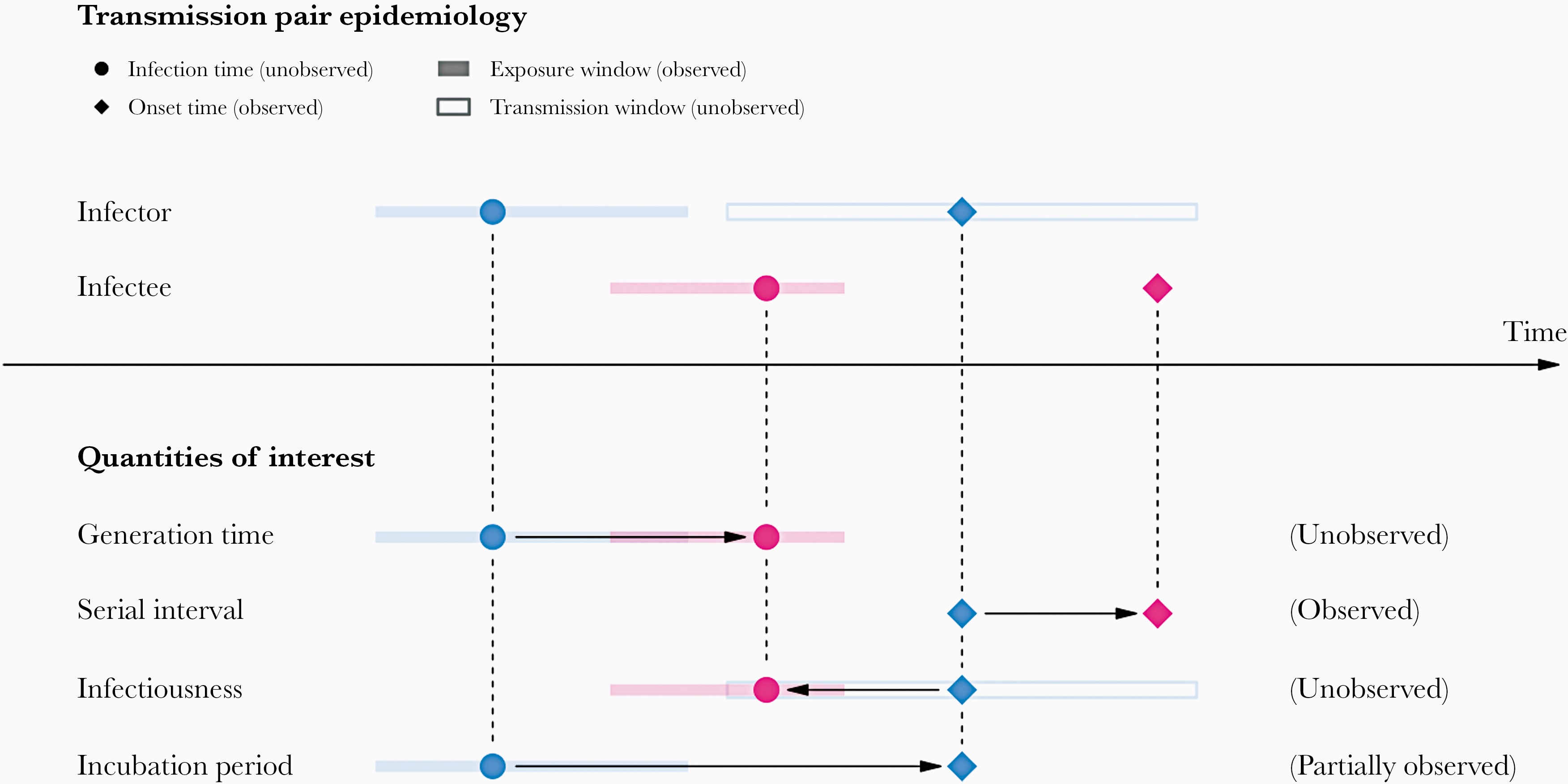
However, using the serial interval as an approximation of the generation time is primarily valid for diseases in which infectiousness starts after symptom onset (Chung Lau et al. 2021). In cases where infectiousness starts before symptom onset, the serial intervals can have negative values, which is the case of a pre-symptomatic transmission (Nishiura et al. (2020)).
Additionally, even if the generation time and serial interval have the same mean, their variance usually differs, propagating bias to the \(R_{t}\) estimation. \(R_{t}\) estimates are sensitive not only to the mean generation time but also to the variance and form of the generation interval distribution (Gostic et al., 2020).
From time periods to probability distributions.
When we calculate the serial interval, we see that not all case pairs have the same time length. We will observe this variability for any case pair and individual time period, including the incubation period and infectious period.
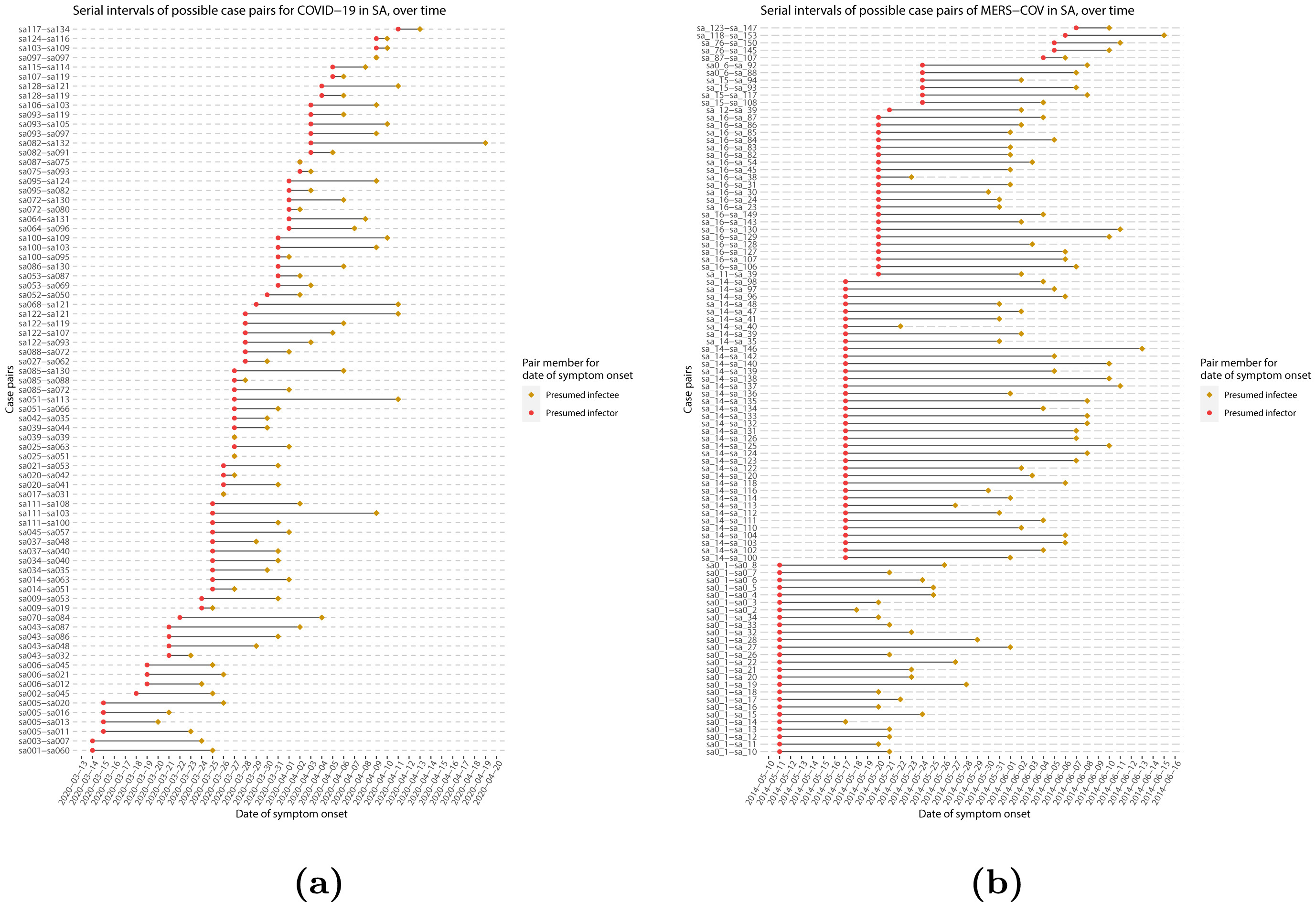
To summarize these data from individual and pair time periods, we can find the statistical distributions that best fit the data (McFarland et al., 2023).
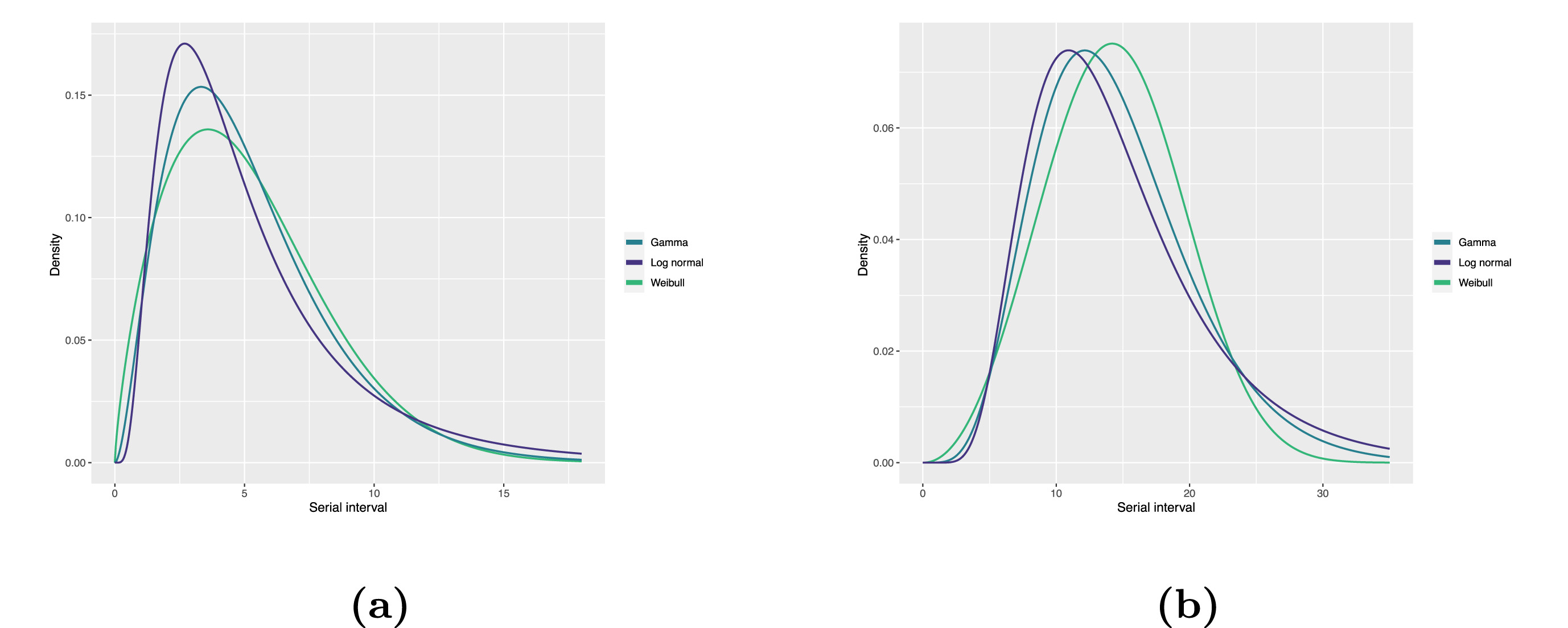
Statistical distributions are summarized in terms of their summary statistics like the location (mean and percentiles) and spread (variance or standard deviation) of the distribution, or with their distribution parameters that inform about the form (shape and rate/scale) of the distribution. These estimated values can be reported with their uncertainty (95% confidence intervals).
| Gamma | mean | shape | rate/scale |
|---|---|---|---|
| MERS-CoV | 14.13(13.9–14.7) | 6.31(4.88–8.52) | 0.43(0.33–0.60) |
| COVID-19 | 5.1(5.0–5.5) | 2.77(2.09–3.88) | 0.53(0.38–0.76) |
| Weibull | mean | shape | rate/scale |
|---|---|---|---|
| MERS-CoV | 14.2(13.3–15.2) | 3.07(2.64–3.63) | 16.1(15.0–17.1) |
| COVID-19 | 5.2(4.6–5.9) | 1.74(1.46–2.11) | 5.83(5.08–6.67) |
| Log normal | mean | mean-log | sd-log |
|---|---|---|---|
| MERS-CoV | 14.08(13.1–15.2) | 2.58(2.50–2.68) | 0.44(0.39–0.5) |
| COVID-19 | 5.2(4.2–6.5) | 1.45(1.31–1.61) | 0.63(0.54–0.74) |
Serial interval
Assume that COVID-19 and SARS have similar reproduction number values and that the serial interval approximates the generation time.
Given the Serial interval of both infections in the figure below:
- Which one would be harder to control?
- Why do you conclude that?
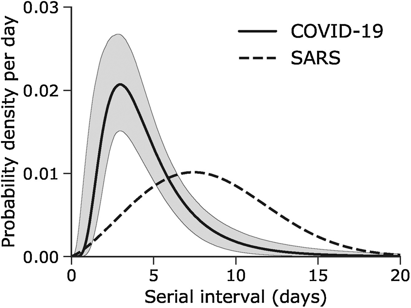
The peak of each curve can inform you about the location of the mean of each distribution. The larger the mean, the larger the serial interval.
Which one would be harder to control?
- COVID-19
Why do you conclude that?
- COVID-19 has the lowest mean serial interval. The approximate mean value for the serial interval of COVID-19 is around four days, and SARS is about seven days. Thus, COVID-19 will likely have newer generations in less time than SARS, assuming similar reproduction numbers.
Extract epidemiological parameters
First, let’s assume that the data set example_confirmed
has COVID-19 observed cases. So, we need to find a reported generation
time for COVID-19 or any other useful parameter for this aim.
Let’s start by looking at how many parameters we have in the
epidemiological distributions database (epidist_db) for the
disease named covid-19:
R
epiparameter::epidist_db(
  disease = "covid"
)
OUTPUT
Returning 27 results that match the criteria (22 are parameterised).
Use subset to filter by entry variables or single_epidist to return a single entry.
To retrieve the short citation for each use the 'get_citation' function
OUTPUT
List of <epidist> objects
  Number of entries in library: 27
  Number of studies in library: 10
  Number of diseases: 1
  Number of delay distributions: 27
  Number of offspring distributions: 0
From the {epiparameter} package, we can use the
epidist_db() function to ask for any disease
and also for a specific epidemiological distribution
(epi_dist).
Let’s ask now how many parameters we have in the epidemiological
distributions database (epidist_db) with the generation
time using the string generation:
R
epiparameter::epidist_db(
  epi_dist = "generation"
)
OUTPUT
Returning 1 results that match the criteria (1 are parameterised).
Use subset to filter by entry variables or single_epidist to return a single entry.
To retrieve the short citation for each use the 'get_citation' function
OUTPUT
Disease: Influenza
Pathogen: Influenza-A-H1N1
Epi Distribution: generation time
Study: Lessler J, Reich N, Cummings D, New York City Department of Health and
Mental Hygiene Swine Influenza Investigation Team (2009). "Outbreak of
2009 Pandemic Influenza A (H1N1) at a New York City School." _The New
England Journal of Medicine_. doi:10.1056/NEJMoa0906089
<https://doi.org/10.1056/NEJMoa0906089>.
Distribution: weibull
Parameters:
  shape: 2.360
  scale: 3.180
Currently, in the library of epidemiological parameters, we have one
generation time entry for Influenza. Considering the
abovementioned considerations, we can look at the serial
intervals for COVID-19.
R
epiparameter::epidist_db(
  disease = "COVID",
  epi_dist = "serial"
)
OUTPUT
Returning 4 results that match the criteria (3 are parameterised).
Use subset to filter by entry variables or single_epidist to return a single entry.
To retrieve the short citation for each use the 'get_citation' function
OUTPUT
[[1]]
Disease: COVID-19
Pathogen: SARS-CoV-2
Epi Distribution: serial interval
Study: Alene M, Yismaw L, Assemie M, Ketema D, Gietaneh W, Birhan T (2021).
"Serial interval and incubation period of COVID-19: a systematic review
and meta-analysis." _BMC Infectious Diseases_.
doi:10.1186/s12879-021-05950-x
<https://doi.org/10.1186/s12879-021-05950-x>.
Parameters: <no parameters>

[[2]]
Disease: COVID-19
Pathogen: SARS-CoV-2
Epi Distribution: serial interval
Study: Nishiura H, Linton N, Akhmetzhanov A (2020). "Serial interval of novel
coronavirus (COVID-19) infections." _International Journal of
Infectious Diseases_. doi:10.1016/j.ijid.2020.02.060
<https://doi.org/10.1016/j.ijid.2020.02.060>.
Distribution: lnorm
Parameters:
  meanlog: 1.386
  sdlog: 0.568

[[3]]
Disease: COVID-19
Pathogen: SARS-CoV-2
Epi Distribution: serial interval
Study: Nishiura H, Linton N, Akhmetzhanov A (2020). "Serial interval of novel
coronavirus (COVID-19) infections." _International Journal of
Infectious Diseases_. doi:10.1016/j.ijid.2020.02.060
<https://doi.org/10.1016/j.ijid.2020.02.060>.
Distribution: weibull
Parameters:
  shape: 2.203
  scale: 5.420

[[4]]
Disease: COVID-19
Pathogen: SARS-CoV-2
Epi Distribution: serial interval
Study: Yang L, Dai J, Zhao J, Wang Y, Deng P, Wang J (2020). "Estimation of
incubation period and serial interval of COVID-19: analysis of 178
cases and 131 transmission chains in Hubei province, China."
_Epidemiology and Infection_. doi:10.1017/S0950268820001338
<https://doi.org/10.1017/S0950268820001338>.
Distribution: norm
Parameters:
  mean: 4.600
  sd: 4.400

attr(,"class")
[1] "multi_epidist"
CASE-INSENSITIVE
epidist_db is case-insensitive.
This means that you can use strings with letters in upper or lower case
indistinctly.
We get more than one epidemiological delay. To summarize this view
and get the column names from the underlying parameter dataset, we can
add the epiparameter::list_distributions() function to the
previous code using the pipe %>%:
R
epiparameter::epidist_db(
  disease = "covid",
  epi_dist = "serial"
) %>%
  epiparameter::list_distributions()
OUTPUT
Returning 4 results that match the criteria (3 are parameterised).
Use subset to filter by entry variables or single_epidist to return a single entry.
To retrieve the short citation for each use the 'get_citation' function
OUTPUT
   disease epi_distribution prob_distribution       author year
1 COVID-19  serial interval              <NA> Muluneh .... 2021
2 COVID-19  serial interval             lnorm Hiroshi .... 2020
3 COVID-19  serial interval           weibull Hiroshi .... 2020
4 COVID-19  serial interval              norm Lin Yang.... 2020
Ebola’s incubation periods
Take 5 minutes:
How many delay distributions are for the Ebola disease?
How many delay distributions are for the incubation period of Ebola?
Explore the library and find the disease with the delay distribution of your interest! Do you recognize the paper?
The {epiparameter} combo of epidist_db()
plus list_distributions() list all the entries by:
- disease,
- epidemiological distribution,
- the type of the probability distribution,
- author of the study, and
- year of study.
R
# 16 delays distributions
epiparameter::epidist_db(
  disease = "ebola"
)

# 5 delay distributions are for the incubation period
epiparameter::epidist_db(
  disease = "ebola",
  epi_dist = "incubation"
)
Now, from the output of epiparameter::epidist_db(), What
is an offspring
distribution?
Select a single distribution
The epiparameter::epidist_db() function works as a
filtering or subset function. Let’s use the author argument
to filter Hiroshi Nishiura parameters:
R
epiparameter::epidist_db(
  disease = "covid",
  epi_dist = "serial",
  author = "Hiroshi"
) %>%
  epiparameter::list_distributions()
OUTPUT
Returning 2 results that match the criteria (2 are parameterised).
Use subset to filter by entry variables or single_epidist to return a single entry.
To retrieve the short citation for each use the 'get_citation' function
OUTPUT
   disease epi_distribution prob_distribution       author year
1 COVID-19  serial interval             lnorm Hiroshi .... 2020
2 COVID-19  serial interval           weibull Hiroshi .... 2020
We still get more than one epidemiological parameter. We can set the
single_epidist argument to TRUE to only
one:
R
epiparameter::epidist_db(
  disease = "covid",
  epi_dist = "serial",
  author = "Hiroshi",
  single_epidist = TRUE
)
OUTPUT
Using Nishiura H, Linton N, Akhmetzhanov A (2020). "Serial interval of novel
coronavirus (COVID-19) infections." _International Journal of
Infectious Diseases_. doi:10.1016/j.ijid.2020.02.060
<https://doi.org/10.1016/j.ijid.2020.02.060>..
To retrieve the short citation use the 'get_citation' function
OUTPUT
Disease: COVID-19
Pathogen: SARS-CoV-2
Epi Distribution: serial interval
Study: Nishiura H, Linton N, Akhmetzhanov A (2020). "Serial interval of novel
coronavirus (COVID-19) infections." _International Journal of
Infectious Diseases_. doi:10.1016/j.ijid.2020.02.060
<https://doi.org/10.1016/j.ijid.2020.02.060>.
Distribution: lnorm
Parameters:
  meanlog: 1.386
  sdlog: 0.568
How does single_epidist
works?
Looking at the help documentation for
?epiparameter::epidist_db():
- If multiple entries match the arguments supplied and
single_epidist = TRUE, - Then, the parameterised
<epidist> with the largest sample size will be returned. - If multiple entries are equal after this sorting, the first entry will be returned.
What does a parametrised <epidist> is? Look at
?is_parameterised.
Now, we have an epidemiological parameter we can reuse! We can
replace the numbers we plug into EpiNow2::dist_spec().
Let’s assign this <epidist> class object to the
covid_serialint object.
R
covid_serialint <-
  epiparameter::epidist_db(
    disease = "covid",
    epi_dist = "serial",
    author = "Nishiura",
    single_epidist = TRUE
  )
OUTPUT
Using Nishiura H, Linton N, Akhmetzhanov A (2020). "Serial interval of novel
coronavirus (COVID-19) infections." _International Journal of
Infectious Diseases_. doi:10.1016/j.ijid.2020.02.060
<https://doi.org/10.1016/j.ijid.2020.02.060>..
To retrieve the short citation use the 'get_citation' function
R
covid_serialint
OUTPUT
Disease: COVID-19
Pathogen: SARS-CoV-2
Epi Distribution: serial interval
Study: Nishiura H, Linton N, Akhmetzhanov A (2020). "Serial interval of novel
coronavirus (COVID-19) infections." _International Journal of
Infectious Diseases_. doi:10.1016/j.ijid.2020.02.060
<https://doi.org/10.1016/j.ijid.2020.02.060>.
Distribution: lnorm
Parameters:
  meanlog: 1.386
  sdlog: 0.568
Ebola’s incubation period
Take 2 minutes:
- What type of distribution has the incubation period of Ebola with the highest sample size?
- How would you access to the sample size of the other studies in the
<multi_epidist>class object?
The {epiparameter} combo of epidist_db()
plus list_distributions() list all the entries by:
- disease,
- epidemiological distribution,
- the type of the probability distribution,
- author of the study, and
- year of study.
This is a <multi_epidist> class object:
R
epiparameter::epidist_db(
  disease = "ebola",
  epi_dist = "incubation"
)
R
# the distribution with the highest sample size has a gamma distribution
epiparameter::epidist_db(
  disease = "ebola",
  epi_dist = "incubation",
  single_epidist = TRUE
)
To access the sample_size, review an issue
reported in the GitHub repository of the {epiparameter}
package.
Extract the summary statistics
We can get the mean and standard deviation
(sd) from this <epidist> diving into the
summary_stats object:
R
# get the mean
covid_serialint$summary_stats$mean
OUTPUT
[1] 4.7How to get the sd and other
nested elements?
Take 1 minute to:
Get the
sdof the epidemiological distribution.Find the
sample_sizeused in the study.Explore all the other nested elements within the
<epidist>object.
Share about:
- What elements do you find useful for your analysis?
- What other elements would you like to see in this object? How?
R
# get the sd
covid_serialint$summary_stats$sd

# get the sample_size
covid_serialint$metadata$sample_size
An interesting element is the method_assess nested
entry, which refers to the methods used by the study authors to assess
for bias while estimating the serial interval distribution.
R
covid_serialint$method_assess
OUTPUT
$censored
[1] TRUE

$right_truncated
[1] TRUE

$phase_bias_adjusted
[1] FALSE
We will explore these concepts at the end!
Ebola’s severity parameter
A severity parameter like the duration of hospitalization could add to the information needed about the bed capacity in response to an outbreak (Cori et al., 2017).
For Ebola:
- what is a reported point estimate and uncertainty of the mean duration of health-care and case isolation?
An informative delay measures the time from symptom onset to recovery or death.
R
# one way to get the list of all the available parameters
epidist_db(disease = "all") %>%
  list_distributions() %>%
  as_tibble() %>%
  distinct(epi_distribution)

ebola_severity <- epidist_db(
  disease = "ebola",
  epi_dist = "onset to discharge"
)

# point estimate
ebola_severity$summary_stats$mean
# 95% confidence intervals
ebola_severity$summary_stats$mean_ci
# limits of the confidence intervals
ebola_severity$summary_stats$mean_ci_limits
Continuous distributions
The following output has four entries with different content in the
probability distribution
(prob_distribution) column:
R
distribution <-
  epiparameter::epidist_db(
    disease = "covid",
    epi_dist = "serial"
  )
OUTPUT
Returning 4 results that match the criteria (3 are parameterised).
Use subset to filter by entry variables or single_epidist to return a single entry.
To retrieve the short citation for each use the 'get_citation' function
R
distribution %>%
  list_distributions()
OUTPUT
   disease epi_distribution prob_distribution       author year
1 COVID-19  serial interval              <NA> Muluneh .... 2021
2 COVID-19  serial interval             lnorm Hiroshi .... 2020
3 COVID-19  serial interval           weibull Hiroshi .... 2020
4 COVID-19  serial interval              norm Lin Yang.... 2020
Entries with a missing value (<NA>) in the
prob_distribution column are non-parameterised
entries. They have summary statistics but no probability distribution.
Compare these two outputs:
R
distribution[[1]]$summary_stats
distribution[[1]]$prob_dist
As detailed in ?is_parameterised, a parameterised
distribution is the entry that has a probability distribution associated
with it provided by an inference_method as shown in
metadata:
R
distribution[[1]]$metadata$inference_method
distribution[[2]]$metadata$inference_method
distribution[[4]]$metadata$inference_method
In the epiparameter::list_distributions() output, we can
also find different types of probability distributions (e.g.,
Log-normal, Weibull, Normal).
R
distribution %>%
  list_distributions()
OUTPUT
disease epi_distribution prob_distribution author year
1 COVID-19 serial interval <NA> Muluneh .... 2021
2 COVID-19 serial interval lnorm Hiroshi .... 2020
3 COVID-19 serial interval weibull Hiroshi .... 2020
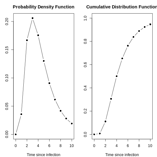
4 COVID-19 serial interval norm Lin Yang.... 2020In {epiparameter}, you will mostly find
continuous distributions like these. You can visualize
any of them with the plot() function and access to:
- the Probability Density Function (PDF) and
- the Cumulative Distribution Function (CDF).
R
plot(distribution[[2]])
With the day_range argument, you can change the length
or number of days in the x axis. Explore what it look
like:
R
plot(distribution[[2]], day_range = 0:20)
The distribution Zoo
Explore this shinyapp called The Distribution Zoo!
Follow these steps to reproduce the form of the
covid_serialint distribution:
- Access to https://ben18785.shinyapps.io/distribution-zoo/ shinyapp website,
- Go to the left panel,
- Keep the Category of distribution:
Continuous Univariate, - Select a new Type of distribution:
Log-Normal, - Move the sliders, i.e. the graphical control
element that allows you to adjust a value by moving a handle along a
horizontal track or bar to the
covid_serialintparameters.
Replicate these with the distribution object and all its
list elements: 2, 3, and 4.
Explore how the shape of a distribution changes when its parameters
change.
Share about:
- What other features of the website do you find helpful?
Distribution functions
In R, all the statistical distributions have functions to access the:
- Probability Density function (PDF),
- Cumulative Distribution function (CDF),
- Quantile function, and
- Random values from the given distribution.
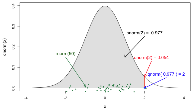
If you need it, read in detail about the R probability functions for the normal distribution, each of its definitions and identify in which part of a distribution they are located!
If you look at ?stats::Distributions, each type of
distribution has a unique set of functions. However,
{epiparameter} gives you the same four functions to access
each of the values above for any <epidist> object you
want!
R
# plot this to have a visual reference
plot(covid_serialint, day_range = 0:20)
R
# the density value at quantile value of 10 (days)
density(covid_serialint, at = 10)
OUTPUT
[1] 0.01911607R
# the cumulative probability at quantile value of 10 (days)
cdf(covid_serialint, q = 10)
OUTPUT
[1] 0.9466605R
# the quantile value (day) at a cumulative probability of 60%
quantile(covid_serialint, p = 0.6)
OUTPUT
[1] 4.618906R
# generate 10 random values (days) given
# the distribution family and its parameters
generate(covid_serialint, times = 10)
OUTPUT
 [1] 2.271797 5.917676 6.223395 6.321504 1.785465 4.854480 2.087282 3.985876
 [9] 3.777108 4.779382
Window for contact tracing and the Serial interval
The serial interval is important in the optimization of contact tracing since it provides a time window for the containment of a disease spread (Fine, 2003). Depending on the serial interval, we can evaluate the need to expand the number of days pre-onset to consider in the contact tracing to include more backwards contacts (Davis et al., 2020).
With the COVID-19 serial interval (covid_serialint)
calculate:
- How much more of the backward cases could be captured if the contact tracing method considered contacts up to 6 days pre-onset compared to 2 days pre-onset?
In Figure 5 from the R
probability functions for the normal distribution, the shadowed
section represents a cumulative probability of 0.997 for
the quantile value at x = 2.
R
plot(covid_serialint)
R
cdf(covid_serialint, q = 2)
cdf(covid_serialint, q = 6)
Given the COVID-19 serial interval:
A contact tracing method considering contacts up to 2 days pre-onset will capture around 11.1% of backward cases.
If this period is extended to 6 days pre-onset, this could include 76.2% of backward contacts.
If we exchange the question between days and cumulative probability to:
- When considering secondary cases, how many days following the symptom onset of primary cases can we expect 55% of symptom onset to occur?
R
quantile(covid_serialint, p = 0.55)
An interpretation could be:
- The 55% percent of the symptom onset of secondary cases will happen after 4.2 days after the symptom onset of primary cases.
Discretize a continuous distribution
We are getting closer to the end! EpiNow2::dist_spec()
still needs a maximum value (max).
One way to do this is to get the quantile value for the
distribution’s 99.9th percentile or 0.999 cumulative
probability. For this, we need access to the set of distribution
functions for our <epidist> object.
We can use the set of distribution functions for a
continuous distribution (as above). However, these values will
be continuous numbers. We can discretize the
continuous distribution stored in our <epidist>
object to get discrete values from a continuous distribution.
When we epiparameter::discretise() the continuous
distribution we get a discrete(-ized) distribution:
R
covid_serialint_discrete <-
  epiparameter::discretise(covid_serialint)

covid_serialint_discrete
OUTPUT
Disease: COVID-19
Pathogen: SARS-CoV-2
Epi Distribution: serial interval
Study: Nishiura H, Linton N, Akhmetzhanov A (2020). "Serial interval of novel
coronavirus (COVID-19) infections." _International Journal of
Infectious Diseases_. doi:10.1016/j.ijid.2020.02.060
<https://doi.org/10.1016/j.ijid.2020.02.060>.
Distribution: discrete lnorm
Parameters:
  meanlog: 1.386
  sdlog: 0.568
We identify this change in the Distribution: output line
of the <epidist> object. Take a double check to this
line:
Distribution: discrete lnormWhile for a continuous distribution, we plot the Probability Density Function (PDF), for a discrete distribution, we plot the Probability Mass Function (PMF):
R
# continuous
plot(covid_serialint)

# discrete
plot(covid_serialint_discrete)
To finally get a max value, let’s access the quantile
value of the 99.9th percentile or 0.999 probability of the
distribution with the prob_dist$q notation, similarly to
how we access the summary_stats values.
R
covid_serialint_discrete_max <-
  covid_serialint_discrete$prob_dist$q(p = 0.999)
Lenght of quarantine and Incubation period
The incubation period distribution is a useful delay to assess the length of active monitoring or quarantine (Lauer et al., 2020). Similarly, delays from symptom onset to recovery (or death) will determine the required duration of health-care and case isolation (Cori et al., 2017).
Calculate:
- Within what exact time frame do 99% of individuals who develop COVID-19 symptoms exhibit them after infection?
What delay distribution measures the time between infection and the onset of symptoms?
The probability function for <epidist>
discrete distributions differ from the
continuous ones!
R
# plot to have a visual reference
plot(covid_serialint_discrete, day_range = 0:20)

# density value at quantile value 10 (day)
covid_serialint_discrete$prob_dist$d(10)

# cumulative probability at quantile value 10 (day)
covid_serialint_discrete$prob_dist$cdf(10)

# In what quantile value (days) do we have the 60% cumulative probability?
covid_serialint_discrete$prob_dist$q(0.6)

# generate random values
covid_serialint_discrete$prob_dist$r(10)
R
covid_incubation <-
  epiparameter::epidist_db(
    disease = "covid",
    epi_dist = "incubation",
    single_epidist = TRUE
  )

covid_incubation_discrete <- epiparameter::discretise(covid_incubation)

covid_incubation_discrete$prob_dist$q(0.99)
99% of those who develop COVID-19 symptoms will do so within 16 days of infection.
Now, Is this result expected in epidemiological terms?
From a maximum value with $prob_dist$q(), we can create
a sequence of quantile values as a numeric vector and map density values
for each:
R
# create a discrete distribution visualization
# from a maximum value from the distribution
covid_serialint_discrete$prob_dist$q(0.999) %>%
  # generate quantile values
  # as a sequence for each natural number
  seq(1L, to = ., by = 1L) %>%
  # coerce numeric vector to data frame
  as_tibble_col(column_name = "quantile_values") %>%
  mutate(
    # map density values
    # for each quantile in the density function
    density_values =
      covid_serialint_discrete$prob_dist$d(quantile_values)
  ) %>%
  # create plot
  ggplot(
    aes(
      x = quantile_values,
      y = density_values
    )
  ) +
  geom_col()
Plug-in {epiparameter} to {EpiNow2}
Now we can plug everything into the EpiNow2::dist_spec()
function!
R
serial_interval_covid <-
  dist_spec(
    mean = covid_serialint$summary_stats$mean,
    sd = covid_serialint$summary_stats$sd,
    max = covid_serialint_discrete_max,
    distribution = "lognormal"
  )

serial_interval_covid
OUTPUT
Fixed distribution with PMF [0.18 0.11 0.08 0.066 0.057 0.05 0.045 0.041 0.037 0.034 0.032 0.03 0.028 0.027 0.025 0.024 0.023 0.022 0.021 0.02 0.019 0.019 0.018]Warning
Using the serial interval instead of the generation time is an alternative that can propagate bias in your estimates, even more so in diseases with reported pre-symptomatic transmission.
Let’s replace the generation_time input we used for
EpiNow2::epinow().
R
epinow_estimates <- epinow(
  # cases
  reported_cases = example_confirmed[1:60],
  # delays
  generation_time = generation_time_opts(serial_interval_covid),
  # computation
  stan = stan_opts(
    cores = 4, samples = 1000, chains = 3,
    control = list(adapt_delta = 0.99)
  )
)

base::plot(epinow_estimates)
Ebola’s effective reproduction number
Download and read the Ebola dataset:
- Reuse one epidemiological parameter to estimate the effective reproduction number for the Ebola dataset.
- Why did you choose that parameter?
To calculate the \(R_t\), we need:
- data set with confirmed cases per day and
- one key delay distribution
Key functions we applied in this episode are:
epidist_db()list_distributions()discretise()- probability functions for continuous and discrete distributions
R
# read data
# e.g.: if path to file is data/raw-data/ebola_cases.csv then:
ebola_confirmed <-
  read_csv(here::here("data", "raw-data", "ebola_cases.csv"))

# list distributions
epidist_db(disease = "ebola") %>%
  list_distributions()

# subset one distribution
ebola_serial <- epidist_db(
  disease = "ebola",
  epi_dist = "serial",
  single_epidist = TRUE
)

ebola_serial_discrete <- discretise(ebola_serial)

serial_interval_ebola <-
  dist_spec(
    mean = ebola_serial$summary_stats$mean,
    sd = ebola_serial$summary_stats$sd,
    max = ebola_serial_discrete$prob_dist$q(p = 0.999),
    distribution = "gamma"
  )

# name of the type of distribution
# only for the discretised distribution
ebola_serial_discrete$prob_dist$name

epinow_estimates <- epinow(
  # cases
  reported_cases = ebola_confirmed,
  # delays
  generation_time = generation_time_opts(serial_interval_ebola),
  # computation
  stan = stan_opts(
    cores = 4, samples = 1000, chains = 3,
    control = list(adapt_delta = 0.99)
  )
)

plot(epinow_estimates)
Adjusting for reporting delays
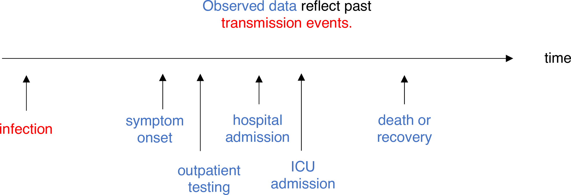
Estimating \(R_t\) requires data on the daily number of new infections. Due to lags in the development of detectable viral loads, symptom onset, seeking care, and reporting, these numbers are not readily available. All observations reflect transmission events from some time in the past. In other words, if \(d\) is the delay from infection to observation, then observations at time \(t\) inform \(R_{t−d}\), not \(R_t\). (Gostic et al., 2020)
The delay distribution could be inferred jointly with the underlying times of infection or estimated as the sum of the incubation period distribution and the distribution of delays from symptom onset to observation from line list data (reporting delay).
For EpiNow2, we can specify these two complementary
delay distributions in the delays argument.
Reuse an Incubation period for COVID-19
Use {epiparameter} to:
- Find an incubation period for COVID-19.
- Add our last
epinow()code chunk using thedelaysargument and thedelay_opts()helper function.
The delays argument and the delay_opts()
helper function are analogous to the generation_time
argument and the generation_time_opts() helper
function.
R
epinow_estimates <- epinow(
  # cases
  reported_cases = example_confirmed[1:60],
  # delays
  generation_time = generation_time_opts(serial_interval_covid),
  delays = delay_opts(incubation_time_covid),
  # computation
  stan = stan_opts(
    cores = 4, samples = 1000, chains = 3,
    control = list(adapt_delta = 0.99)
  )
)
R
covid_incubation <- epiparameter::epidist_db(
  disease = "covid",
  epi_dist = "incubation",
  author = "Natalie",
  single_epidist = TRUE
)

covid_incubation

covid_incubation_discrete <- epiparameter::discretise(covid_incubation)

incubation_time_covid <- dist_spec(
  mean = covid_incubation$summary_stats$mean,
  sd = covid_incubation$summary_stats$sd,
  max = covid_incubation_discrete$prob_dist$q(p = 0.999),
  distribution = "lognormal"
)

epinow_estimates <- epinow(
  # cases
  reported_cases = example_confirmed[1:60],
  # delays
  generation_time = generation_time_opts(serial_interval_covid),
  delays = delay_opts(incubation_time_covid),
  # computation
  stan = stan_opts(
    cores = 4, samples = 1000, chains = 3,
    control = list(adapt_delta = 0.99)
  )
)

base::plot(epinow_estimates)
After adding the incubation period, discuss:
- Does the retrospective trend of forecast change?
- Has the uncertainty changed?
- How would you explain or interpret any of these changes?
Ebola’s effective reproduction number was adjusted by reporting delays
Using the same Ebola dataset:
- Reuse one additional epidemiological parameter for the
delaysargument inEpiNow2::epinow(). - Estimate the effective reproduction number using
EpiNow2::epinow(). - Why did you choose that parameter?
We can use two complementary delay distributions to estimate the \(R_t\) at time \(t\).
R
# read data
# e.g.: if path to file is data/raw-data/ebola_cases.csv then:
ebola_confirmed <-
  read_csv(here::here("data", "raw-data", "ebola_cases.csv"))

# list distributions
epidist_db(disease = "ebola") %>%
  list_distributions()

# subset one distribution for the generation time
ebola_serial <- epidist_db(
  disease = "ebola",
  epi_dist = "serial",
  single_epidist = TRUE
)

ebola_serial_discrete <- discretise(ebola_serial)

serial_interval_ebola <-
  dist_spec(
    mean = ebola_serial$summary_stats$mean,
    sd = ebola_serial$summary_stats$sd,
    max = ebola_serial_discrete$prob_dist$q(p = 0.999),
    distribution = "gamma"
  )

# subset one distribution for delay of the incubation period
ebola_incubation <- epidist_db(
  disease = "ebola",
  epi_dist = "incubation",
  single_epidist = TRUE
)

ebola_incubation_discrete <- discretise(ebola_incubation)

incubation_period_ebola <-
  dist_spec(
    mean = ebola_incubation$summary_stats$mean,
    sd = ebola_incubation$summary_stats$sd,
    max = ebola_incubation_discrete$prob_dist$q(p = 0.999),
    distribution = "gamma"
  )

epinow_estimates <- epinow(
  # cases
  reported_cases = ebola_confirmed,
  # delays
  generation_time = generation_time_opts(serial_interval_ebola),
  delays = delay_opts(incubation_period_ebola),
  # computation
  stan = stan_opts(
    cores = 4, samples = 1000, chains = 3,
    control = list(adapt_delta = 0.99)
  )
)

plot(epinow_estimates)
Extract parameters
Use the influenza_england_1978_school from the
outbreaks package to calculate the effective reproduction
number.
How to get the mean and standard deviation from a generation time with median and quantiles as summary statistics?
- Look at how to extract parameters from
{epiparameter}vignette on parameter extraction and conversion
R
# What parameters are available for Influenza?
epidist_db(disease = "influenza") %>%
  list_distributions() %>%
  as_tibble() %>%
  count(epi_distribution)

influenza_generation <-
  epidist_db(
    disease = "influenza",
    epi_dist = "generation"
  )

influenza_generation_discrete <-
  discretise(influenza_generation)

# problem
# the summary statistics do not have mean and sd
influenza_generation$summary_stats
influenza_generation$summary_stats$median
influenza_generation$summary_stats$quantiles

# solution
# extract parameters from percentiles
influenza_extracted <- extract_param(
  type = "percentiles",
  values = c(influenza_generation$summary_stats$quantiles[1],
             influenza_generation$summary_stats$quantiles[2]),
  distribution = "lnorm",
  percentiles = c(0.05, 0.95)
)

influenza_extracted

generation_time_influenza <-
  dist_spec(
    mean = influenza_extracted[1],
    sd = influenza_extracted[2],
    max = influenza_generation_discrete$prob_dist$q(p = 0.999),
    distribution = "lognormal"
  )

influenza_cleaned <-
  outbreaks::influenza_england_1978_school %>%
  select(date, confirm = in_bed)

epinow_estimates <- epinow(
  # cases
  reported_cases = influenza_cleaned,
  # delays
  generation_time = generation_time_opts(generation_time_influenza),
  # computation
  stan = stan_opts(
    cores = 4, samples = 1000, chains = 3,
    control = list(adapt_delta = 0.99)
  )
)

plot(epinow_estimates)
When to reuse? When to estimate?
In the early stage of an outbreak, we can rely on reusing parameters for known pathogens to unknown ones, like for the Disease X, a pathogen currently unknown to cause human disease and potentially cause a serious international epidemic (WHO, 2018).
But when data from lines list paired with contact tracing is available, we can estimate the key delay distributions that best fit our data. These will help us to inform, compare and update any previous estimate about questions like:
- How long should contacts be followed?
- What is the required duration of contact tracing?
- How long should cases be isolated to reduce transmission?
However, the methods to accurately estimate delays like the generation interval from contact tracing data involve adjusting for biases like censoring, right truncation and epidemic phase bias. (Gostic et al., 2020)
We can identify what entries in the {epiparameter}
library assessed for these biases in their methodology with the
method_assess nested entry:
R
covid_serialint$method_assess
OUTPUT
$censored
[1] TRUE

$right_truncated
[1] TRUE

$phase_bias_adjusted
[1] FALSE
How to estimate delay distributions for Disease X?
Refer to this excellent tutorial on estimating the serial interval and incubation period of Disease X accounting for censoring using Bayesian inference with packages like rstan and coarseDataTools.
- Tutorial in English: https://rpubs.com/tracelac/diseaseX
- Tutorial en Español: https://epiverse-trace.github.io/epimodelac/EnfermedadX.html
The lengths of the Serial interval and Incubation period determine the type of disease transmission.
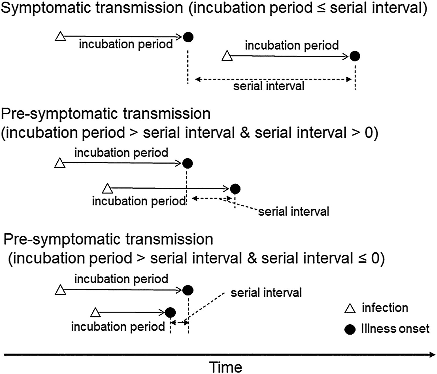
Estimating the proportion of pre-symptomatic infections, or the extent to which infectiousness precedes symptom onset will determine the effectiveness of contact tracing and the feasibility of controlling an outbreak (Fraser et al., 2004 and Hellewell et al., 2020).
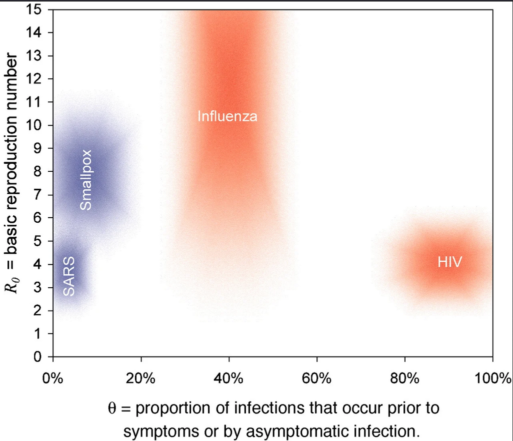
Meta-analysis on the proportion of pre-symptomatic and asymptomatic transmission in SARS-CoV-2 found limitations of the evidence given high heterogeneity and high risk of selection and information bias between studies (Buitrago-Garcia et al., 2022). This is a call to action to improve the Outbreak Analytic pipelines to use and reuse in the early phase of an outbreak.
What type of transmission?
Compare the serial interval and incubation period of Influenza and MERS:
- What type of transmission has Influenza?
- What type of transmission has MERS?
- Do these results correlate with the available evidence?
For types of transmission, we refer to infections with symptomatic or pre-symptomatic transmission.
Key functions:
epidist_db()epidist$summary_stats$
In this solution we use purrr::pluck() to extract
elements within the summary_stats object which is of class
list.
R
# pre-symptomatic transmission
epidist_db(
  disease = "influenza",
  epi_dist = "incubation",
  single_epidist = TRUE
) %>%
  pluck("summary_stats") %>%
  pluck("mean")

epidist_db(
  disease = "influenza",
  epi_dist = "serial",
  single_epidist = TRUE
) %>%
  pluck("summary_stats") %>%
  pluck("mean")

# symptomatic transmission
epidist_db(
  disease = "mers",
  epi_dist = "incubation",
  single_epidist = TRUE
) %>%
  pluck("summary_stats") %>%
  pluck("median")

epidist_db(
  disease = "mers",
  epi_dist = "serial",
  single_epidist = TRUE
) %>%
  pluck("summary_stats") %>%
  pluck("mean")
R
# pre-symptomatic transmission
epidist_db(
  disease = "covid",
  epi_dist = "incubation",
  author = "Stephen",
  single_epidist = TRUE
) %>%
  pluck("summary_stats") %>%
  pluck("mean")

epidist_db(
  disease = "covid",
  epi_dist = "serial",
  author = "Nishiura",
  single_epidist = TRUE
) %>%
  pluck("summary_stats") %>%
  pluck("mean")

# symptomatic transmission
epidist_db(
  disease = "ebola",
  epi_dist = "incubation",
  single_epidist = TRUE
) %>%
  pluck("summary_stats") %>%
  pluck("mean")

epidist_db(
  disease = "ebola",
  epi_dist = "serial",
  single_epidist = TRUE
) %>%
  pluck("summary_stats") %>%
  pluck("mean")
Key Points
- Use
{epiparameter}to access the systematic review catalogue of epidemiological delay distributions. - Use
epidist_db()to select single delay distributions. - Use
list_distributions()for an overview of multiple delay distributions. - Use
discretise()to convert continuous to discrete delay distributions. - Use
{epiparameter}probability functions for any delay distributions.