Modelling interventions
Last updated on 2024-09-24 | Edit this page
Overview
Questions
- How do I investigate the effect of interventions on disease trajectories?
Objectives
- Add pharmaceutical and non-pharmaceutical interventions to an {epidemics} model
Prerequisites
- Complete tutorial Simulating transmission
Learners should familiarise themselves with following concept dependencies before working through this tutorial:
Outbreak response : Intervention types.
Introduction
Mathematical models can be used to generate trajectories of disease spread under the implementation of interventions at different stages of an outbreak. These predictions can be used to make decisions on what interventions could be implemented to slow down the spread of diseases.
We can assume interventions in mathematical models reduce the values of relevant parameters e.g. reduce transmissibility while in place. Or it may be appropriate to assume individuals are classified into a new disease state, e.g. once vaccinated we assume individuals are no longer susceptible to infection and therefore move to a vaccinated state. In this tutorial, we will introduce how to include three different interventions in model of COVID-19 transmission.
Non-pharmaceutical interventions
Non-pharmaceutical interventions (NPIs) are measures put in place to reduce transmission that do not include the administration of drugs or vaccinations. NPIs aim reduce contact between infectious and susceptible individuals. For example, washing hands, wearing masks and closures of school and workplaces.
We will investigate the effect of interventions on a COVID-19
outbreak using an SEIR model (model_default_cpp() in the R
package {epidemics}). We will set \(R_0 = 2.7\), latent period or preinfectious
period \(= 4\) and the
infectious_period \(= 5.5\) (parameters
adapted from Davies et
al. (2020)). We load a contact matrix with age bins 0-18, 18-65, 65
years and older using socialmixr and assume that one in
every 1 million in each age group is infectious at the start of the
epidemic.
R
polymod <- socialmixr::polymod
contact_data <- socialmixr::contact_matrix(
  polymod,
  countries = "United Kingdom",
  age.limits = c(0, 15, 65),
  symmetric = TRUE
)

# prepare contact matrix
contact_matrix <- t(contact_data$matrix)

# prepare the demography vector
demography_vector <- contact_data$demography$population
names(demography_vector) <- rownames(contact_matrix)

# initial conditions: one in every 1 million is infected
initial_i <- 1e-6
initial_conditions <- c(
  S = 1 - initial_i, E = 0, I = initial_i, R = 0, V = 0
)

# build for all age groups
initial_conditions <- matrix(
  rep(initial_conditions, dim(contact_matrix)[1]),
  ncol = 5, byrow = TRUE
)
rownames(initial_conditions) <- rownames(contact_matrix)

# prepare the population to model as affected by the epidemic
uk_population <- population(
  name = "UK",
  contact_matrix = contact_matrix,
  demography_vector = demography_vector,
  initial_conditions = initial_conditions
)
Effect of school closures on COVID-19 spread
The first NPI we will consider is the effect of school closures on reducing the number of individuals infectious with COVID-19 through time. We assume that a school closure will reduce the frequency of contacts within and between different age groups. We assume that school closures will reduce the contacts between school aged children (aged 0-15) by 0.5, and will cause a small reduction (0.01) in the contacts between adults (aged 15 and over).
To include an intervention in our model we must create an
intervention object. The inputs are the name of the
intervention (name), the type of intervention
(contacts or rate), the start time
(time_begin), the end time (time_end) and the
reduction (reduction). The values of the reduction matrix
are specified in the same order as the age groups in the contact
matrix.
R
rownames(contact_matrix)
OUTPUT
[1] "[0,15)" "[15,65)" "65+" Therefore, we specify
reduction = matrix(c(0.5, 0.01, 0.01)). We assume that the
school closures start on day 50 and are in place for a further 100 days.
Therefore our intervention object is :
R
close_schools <- intervention(
  name = "School closure",
  type = "contacts",
  time_begin = 50,
  time_end = 50 + 100,
  reduction = matrix(c(0.5, 0.01, 0.01))
)
Effect of interventions on contacts
In epidemics, the contact matrix is scaled down by
proportions for the period in which the intervention is in place. To
understand how the reduction is calculated within the model functions,
consider a contact matrix for two age groups with equal number of
contacts:
OUTPUT
     [,1] [,2]
[1,]    1    1
[2,]    1    1
If the reduction is 50% in group 1 and 10% in group 2, the contact matrix during the intervention will be:
OUTPUT
     [,1] [,2]
[1,] 0.25 0.45
[2,] 0.45 0.81
The contacts within group 1 are reduced by 50% twice to accommodate for a 50% reduction in outgoing and incoming contacts (\(1\times 0.5 \times 0.5 = 0.25\)). Similarly, the contacts within group 2 are reduced by 10% twice. The contacts between group 1 and group 2 are reduced by 50% and then by 10% (\(1 \times 0.5 \times 0.9= 0.45\)).
Using transmissibility \(= 2.7/5.5\)
(remember that transmissibility
= \(R_0\)/ infectious period),
infectiousness rate \(1/= 4\) and the
recovery rate \(= 1/5.5\) we run the
model withintervention = list(contacts = close_schools) as
follows :
R
output_school <- model_default_cpp(
  population = uk_population,
  transmissibility = 2.7 / 5.5,
  infectiousness_rate = 1.0 / 4.0,
  recovery_rate = 1.0 / 5.5,
  intervention = list(contacts = close_schools),
  time_end = 300, increment = 1.0
)
To be able to see the effect of our intervention, we also run the
model where there is no intervention, combine the two outputs into one
data frame and then plot the output. Here we plot the total number of
infectious individuals in all age groups using
ggplot2::stat_summary():
R
# run baseline simulation with no intervention
output_baseline <- model_default_cpp(
  population = uk_population,
  transmissibility = 2.7 / 5.5,
  infectiousness_rate = 1.0 / 4.0,
  recovery_rate = 1.0 / 5.5,
  time_end = 300, increment = 1.0
)

# create intervention_type column for plotting
output_school$intervention_type <- "school closure"
output_baseline$intervention_type <- "baseline"
output <- rbind(output_school, output_baseline)

ggplot(data = output[output$compartment == "infectious", ]) +
  aes(
    x = time,
    y = value,
    color = intervention_type,
    linetype = intervention_type
  ) +
  stat_summary(
    fun = "sum",
    geom = "line",
    linewidth = 1
  ) +
  scale_y_continuous(
    labels = scales::comma
  ) +
  labs(
    x = "Simulation time (days)",
    y = "Individuals"
  ) +
  theme_bw(
    base_size = 15
  ) +
  geom_vline(
    xintercept = c(close_schools$time_begin, close_schools$time_end),
    colour = "black",
    linetype = "dashed",
    linewidth = 0.2
  ) +
  annotate(
    geom = "text",
    label = "Schools closed",
    colour = "black",
    x = (close_schools$time_end - close_schools$time_begin) / 2 +
      close_schools$time_begin,
    y = 10,
    angle = 0,
    vjust = "outward"
  )
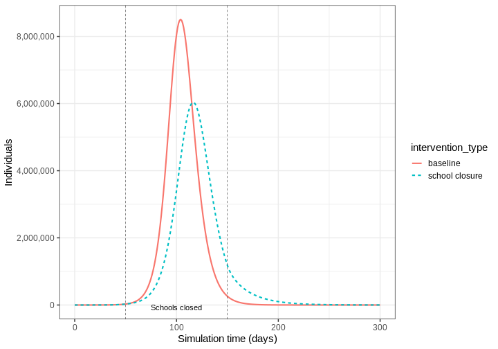 We see that with the intervention in place, the infection still spreads
through the population, though the peak number of infectious individuals
is smaller than the baseline with no intervention in place (solid
line).
We see that with the intervention in place, the infection still spreads
through the population, though the peak number of infectious individuals
is smaller than the baseline with no intervention in place (solid
line).
Effect of mask wearing on COVID-19 spread
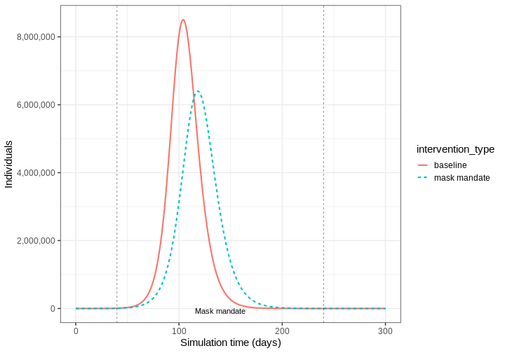
We can model the effect of other NPIs as reducing the value of relevant parameters. For example, we want to investigate the effect of mask wearing on the number of individuals infectious with COVID-19 through time.
We expect that mask wearing will reduce an individual’s infectiousness. As we are using a population based model, we cannot make changes to individual behaviour and so assume that the transmissibility \(\beta\) is reduced by a proportion due to mask wearing in the population. We specify this proportion, \(\theta\) as product of the proportion wearing masks multiplied by the proportion reduction in transmissibility (adapted from Li et al. 2020)
We create an intervention object with type = rate and
reduction = 0.161. Using parameters adapted from Li et al. 2020
we have proportion wearing masks = coverage \(\times\) availability = \(0.54 \times 0.525 = 0.2835\), proportion
reduction in transmissibility = \(0.575\). Therefore, \(\theta = 0.2835 \times 0.575 = 0.163\). We
assume that the mask wearing mandate starts at day 40 and is in place
for 200 days.
R
mask_mandate <- intervention(
  name = "mask mandate",
  type = "rate",
  time_begin = 40,
  time_end = 40 + 200,
  reduction = 0.163
)
To implement this intervention on the parameter \(\beta\), we specify
intervention = list(beta = mask_mandate).
R
output_masks <- model_default_cpp(
  population = uk_population,
  transmissibility = 2.7 / 5.5,
  infectiousness_rate = 1.0 / 4.0,
  recovery_rate = 1.0 / 5.5,
  intervention = list(transmissibility = mask_mandate),
  time_end = 300, increment = 1.0
)
R
# create intervention_type column for plotting
output_masks$intervention_type <- "mask mandate"
output_baseline$intervention_type <- "baseline"
output <- rbind(output_masks, output_baseline)

ggplot(data = output[output$compartment == "infectious", ]) +
  aes(
    x = time,
    y = value,
    color = intervention_type,
    linetype = intervention_type
  ) +
  stat_summary(
    fun = "sum",
    geom = "line",
    linewidth = 1
  ) +
  scale_y_continuous(
    labels = scales::comma
  ) +
  labs(
    x = "Simulation time (days)",
    y = "Individuals"
  ) +
  theme_bw(
    base_size = 15
  ) +
  geom_vline(
    xintercept = c(mask_mandate$time_begin, mask_mandate$time_end),
    colour = "black",
    linetype = "dashed",
    linewidth = 0.2
  ) +
  annotate(
    geom = "text",
    label = "Mask mandate",
    colour = "black",
    x = (mask_mandate$time_end - mask_mandate$time_begin) / 2 +
      mask_mandate$time_begin,
    y = 10,
    angle = 0,
    vjust = "outward"
  )
Intervention types
There are two intervention types for
model_default_cpp(). Rate interventions on model parameters
(transmissibillity \(\beta\), infectiousness_rate
\(\sigma\) and
recovery_rate \(\gamma\))
and contact matrix reductions contacts.
To implement both contact and rate interventions in the same
simulation they must be passed as a list
e.g. intervention = list(transmissibility = mask_mandate, contacts = close_schools).
But if there are multiple interventions that target contact rates, these
must be passed as one contacts input. See the vignette
on modelling overlapping interventions for more detail.
Pharmaceutical interventions
Pharmaceutical interventions (PIs) are measures such as vaccination and mass treatment programs. In the previous section, we assumed that interventions reduced the value of parameter values while the intervention was in place. In the case of vaccination, we assume that after the intervention individuals are no longer susceptible and should be classified into a different disease state. Therefore, we specify the rate at which individuals are vaccinated and track the number of vaccinated individuals through time.
The diagram below shows the SEIRV model implemented using
model_default_cpp() where susceptible individuals are
vaccinated and then move to the \(V\)
class.
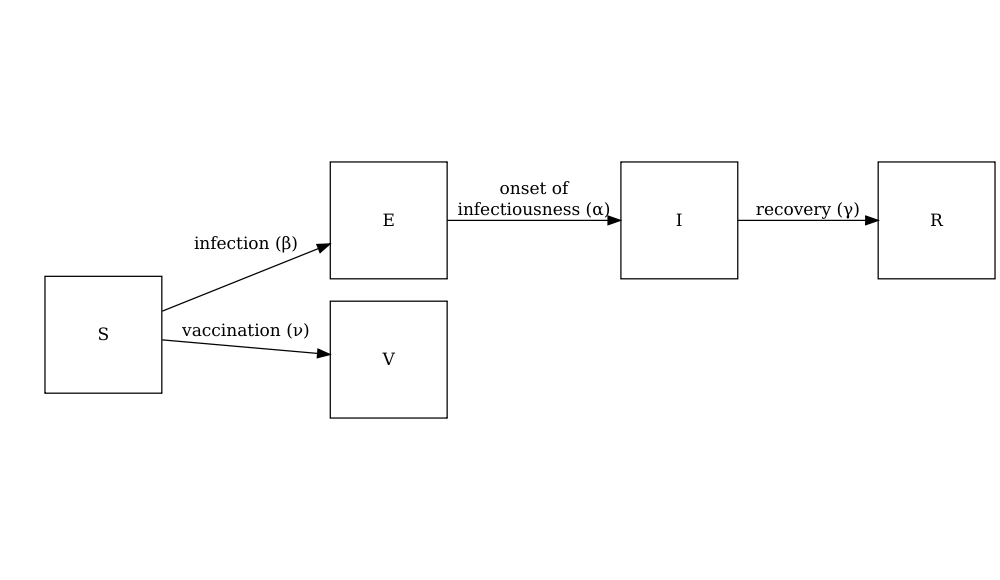
The equations describing this model are as follows:
\[ \begin{aligned} \frac{dS_i}{dt} & = - \beta S_i \sum_j C_{i,j} I_j -\nu_{t} S_i \\ \frac{dE_i}{dt} &= \beta S_i\sum_j C_{i,j} I_j - \alpha E_i \\ \frac{dI_i}{dt} &= \alpha E_i - \gamma I_i \\ \frac{dR_i}{dt} &=\gamma I_i \\ \frac{dV_i}{dt} & =\nu_{i,t} S_i\\ \end{aligned} \] Individuals are vaccinated at an age group (\(i\)) specific time dependent (\(t\)) vaccination rate (\(\nu_{i,t}\)). The SEIR components of these equations are described in the tutorial simulating transmission.
To explore the effect of vaccination we need to create a vaccination
object to pass as an input into model_default_cpp() that
includes an age groups specific vaccination rate nu and age
group specific start and end times of the vaccination program
(time_begin and time_end).
Here we will assume all age groups are vaccinated at the same rate 0.01 and that the vaccination program starts on day 40 and is in place for 150 days.
R
# prepare a vaccination object
vaccinate <- vaccination(
  name = "vaccinate all",
  time_begin = matrix(40, nrow(contact_matrix)),
  time_end = matrix(40 + 150, nrow(contact_matrix)),
  nu = matrix(c(0.01, 0.01, 0.01))
)
We pass our vaccination object using
vaccination = vaccinate:
R
output_vaccinate <- model_default_cpp(
  population = uk_population,
  transmissibility = 2.7 / 5.5,
  infectiousness_rate = 1.0 / 4.0,
  recovery_rate = 1.0 / 5.5,
  vaccination = vaccinate,
  time_end = 300, increment = 1.0
)
Compare interventions
Plot the three interventions vaccination, school closure and mask mandate and the baseline simulation on one plot. Which intervention reduces the peak number of infectious individuals the most?
R
# create intervention_type column for plotting
output_vaccinate$intervention_type <- "vaccination"
output <- rbind(output_school, output_masks, output_vaccinate, output_baseline)

ggplot(data = output[output$compartment == "infectious", ]) +
  aes(
    x = time,
    y = value,
    color = intervention_type,
    linetype = intervention_type
  ) +
  stat_summary(
    fun = "sum",
    geom = "line",
    linewidth = 1
  ) +
  scale_y_continuous(
    labels = scales::comma
  ) +
  labs(
    x = "Simulation time (days)",
    y = "Individuals"
  ) +
  theme_bw(
    base_size = 15
  )
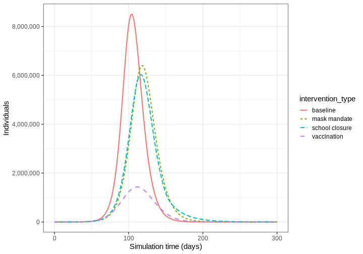
From the plot we see that the peak number of total number of infectious individuals when vaccination is in place is much lower compared to school closures and mask wearing interventions.
Summary
Different types of intervention can be implemented using mathematical modelling. Modelling interventions requires assumptions of which model parameters are affected (e.g. contact matrices, transmissibility), by what magnitude and and what times in the simulation of an outbreak.
The next step is to quantify the effect of an interventions. If you are interested in learning how to compare interventions, please complete the tutorial Comparing public health outcomes of interventions.
Key Points
- The effect of NPIs can be modelled as reducing contact rates between age groups or reducing the transmissibility of infection
- Vaccination can be modelled by assuming individuals move to a different disease state \(V\)