Outbreak analytics pipelines


Figure 1


Figure 2

The outbreak analytics pipeline.

Figure 3


Read delays


Figure 1

Definition of key time periods. From Xiang et al, 2021

Figure 2

Video from the MRC Centre for Global Infectious Disease Analysis, Ep 76. Science In Context - Epi Parameter Review Group with Dr Anne Cori (27-07-2023) at https://youtu.be/VvpYHhFDIjI?si=XiUyjmSV1gKNdrrL

Figure 3

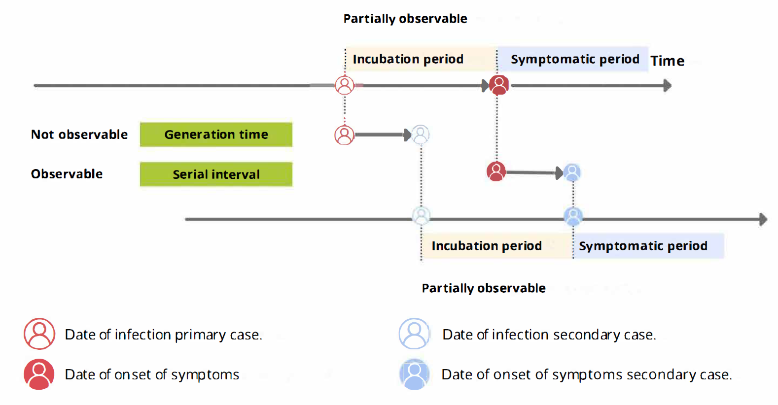
A schematic of the relationship of different time periods of transmission between an infector and an infectee in a transmission pair. Exposure window is defined as the time interval having viral exposure, and transmission window is defined as the time interval for onward transmission with respect to the infection time (Chung Lau et al. 2021).

Figure 4

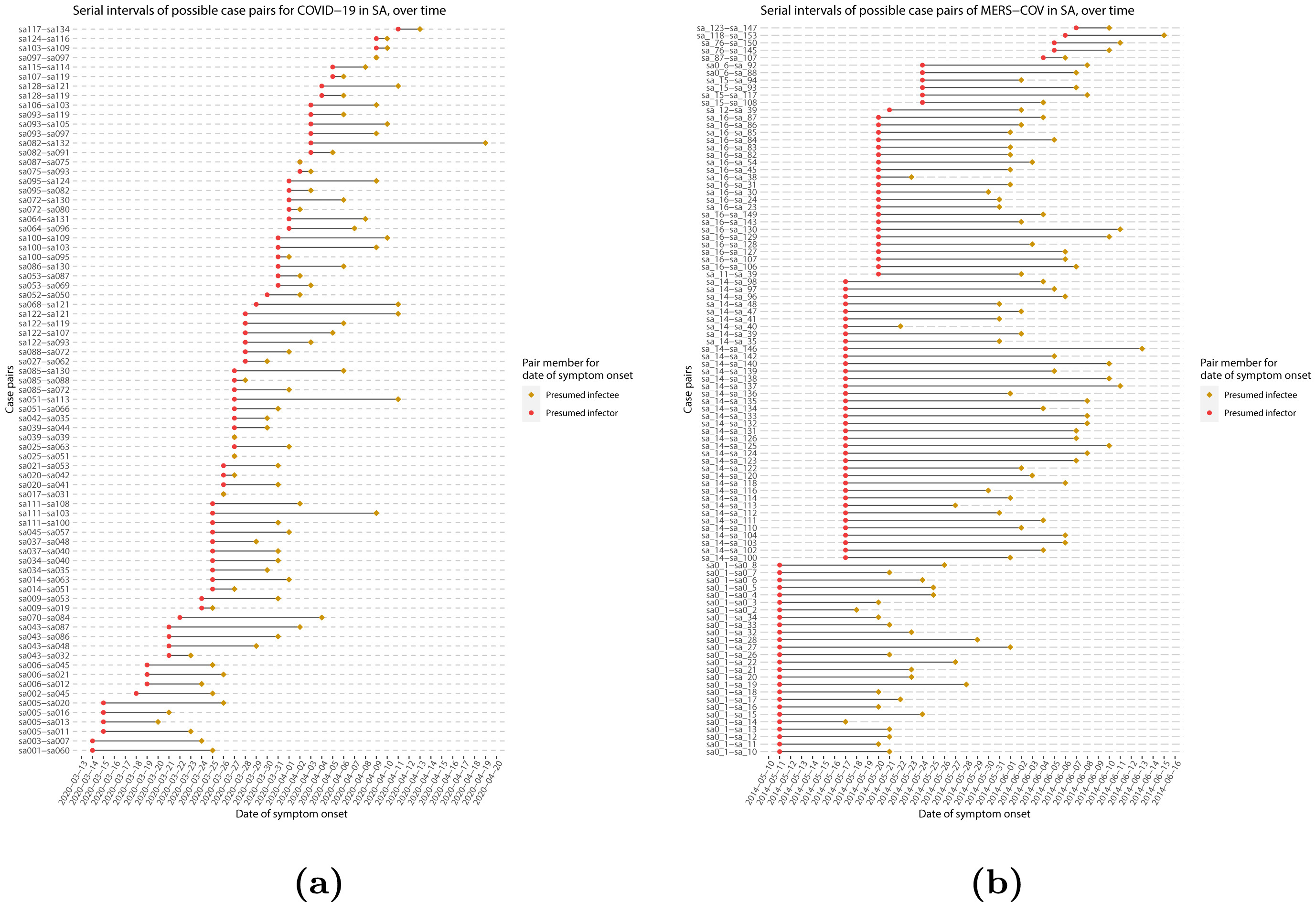
Serial intervals of possible case pairs in (a) COVID-19 and (b) MERS-CoV. Pairs represent a presumed infector and their presumed infectee plotted by date of symptom onset (Althobaity et al., 2022).

Figure 5

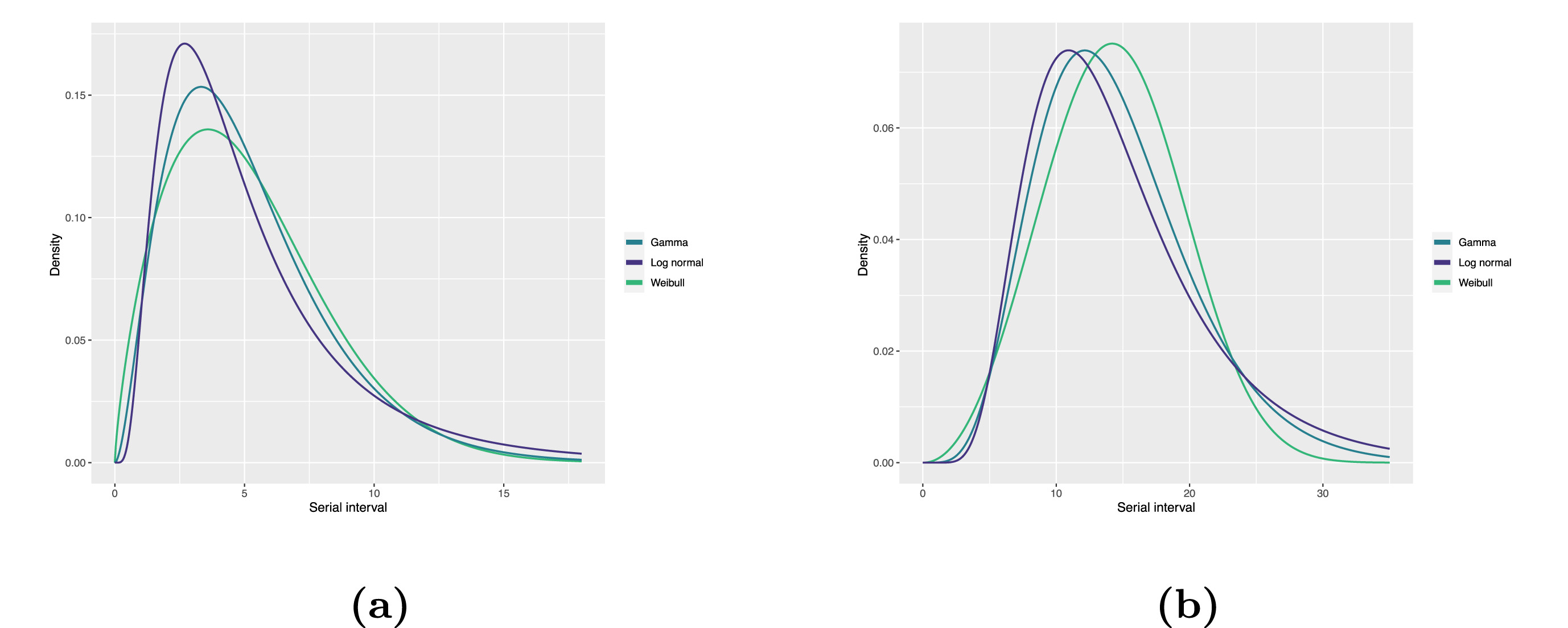
Fitted serial interval distribution for (a) COVID-19 and (b) MERS-CoV based on reported transmission pairs in Saudi Arabia. We fitted three commonly used distributions, Lognormal, Gamma, and Weibull distributions, respectively (Althobaity et al., 2022).

Figure 6

Serial interval of novel coronavirus (COVID-19) infections overlaid with a published distribution of SARS. (Nishiura et al, 2020)

Figure 7


Figure 8

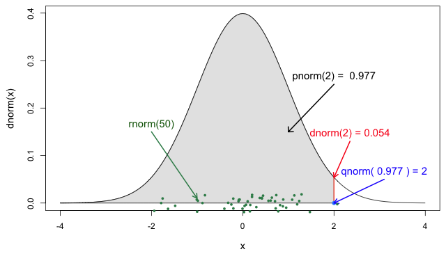
The four probability functions for the normal distribution (Jack Weiss, 2012)

Figure 9

Timeline for chain of disease reporting, the Netherlands. Lab, laboratory; PHA, public health authority. From Marinović et al., 2015

Figure 10

Rt is a measure of transmission at time t. Observations after time t must be adjusted. ICU, intensive care unit. From Gostic et al., 2020

Figure 11

The relationship between the incubation period and serial interval. From Nishiura 2020

Figure 12

Parameter estimates. Plausible ranges for the key parameters R0 and θ (read the main text for sources) for four viral infections of public concern are shown as shaded regions. The size of the shaded area reflects the uncertainties in the parameter estimates. Fraser et al., 2004

Quantifying transmission


Figure 1


Figure 2


Figure 3


Figure 4


Figure 5


Create a short-term forecast


Figure 1


Figure 2


Figure 3


Simulating transmission


Figure 1


Figure 2


Figure 3


Figure 4


Choosing an appropriate model


Figure 1


Figure 2


Figure 3


Figure 4


Modelling interventions


Figure 1

We see that with the intervention in place, the infection still spreads through the population, though the peak number of infectious individuals is smaller than the baseline with no intervention in place (solid line).


Figure 2


Figure 3


Figure 4


Comparing public health outcomes of interventions


Figure 1