Quantifying transmission
Last updated on 2024-09-24 | Edit this page
Estimated time: 30 minutes
Overview
Questions
- How can I estimate key transmission metrics from a time series of case data?
- How can I quantify geographical heterogeneity in these metrics?
Objectives
- Learn how to estimate transmission metrics from a time series of
case data using the R package
EpiNow2
Prerequisites
Learners should familiarise themselves with following concept dependencies before working through this tutorial:
Statistics : probability distributions, principle of Bayesian analysis.
Epidemic theory : Effective reproduction number.
Reminder: the Effective Reproduction Number, \(R_t\)
The basic reproduction number, \(R_0\), is the average number of cases caused by one infectious individual in a entirely susceptible population.
But in an ongoing outbreak, the population does not remain entirely susceptible as those that recover from infection are typically immune. Moreover, there can be changes in behaviour or other factors that affect transmission. When we are interested in monitoring changes in transmission we are therefore more interested in the value of the effective reproduction number, \(R_t\), the average number of cases caused by one infectious individual in the population at time \(t\).
Introduction
Quantifying transmission metrics at the start of an outbreak can give important information on the strength of transmission (reproduction number) and the speed of transmission (growth rate, doubling/halving time). To estimate these key metrics using case data we must account for delays between the date of infections and date of reported cases. In an outbreak situation, data are usually available on reported dates only, therefore we must use estimation methods to account for these delays when trying to understand changes in transmission over time.
In the next tutorials we will focus on how to implement the functions in EpiNow2 to estimate transmission metrics of case data. We will not cover the theoretical background of the models or inference framework, for details on these concepts see the vignette. For more details on the distinction between speed and strength of transmission and implications for control, see Dushoff & Park, 2021.
Bayesian inference
The R package EpiNow2 uses a Bayesian inference framework to
estimate reproduction numbers and infection times based on reporting
dates.
In Bayesian inference, we use prior knowledge (prior distributions) with data (in a likelihood function) to find the posterior probability.
Posterior probability \(\propto\) likelihood \(\times\) prior probability
The first step is to load the EpiNow2 package :
R
library(EpiNow2)
This tutorial illustrates the usage of epinow() to
estimate the time-varying reproduction number and infection times.
Learners should understand the necessary inputs to the model and the
limitations of the model output.
Delay distributions and case data
Case data
To illustrate the functions of EpiNow2 we will use
outbreak data of the start of the COVID-19 pandemic from the United
Kingdom. The data are available in the R package
incidence2.
R
head(incidence2::covidregionaldataUK)
OUTPUT
        date          region region_code cases_new cases_total deaths_new
1 2020-01-30   East Midlands   E12000004        NA          NA         NA
2 2020-01-30 East of England   E12000006        NA          NA         NA
3 2020-01-30         England   E92000001         2           2         NA
4 2020-01-30          London   E12000007        NA          NA         NA
5 2020-01-30      North East   E12000001        NA          NA         NA
6 2020-01-30      North West   E12000002        NA          NA         NA
  deaths_total recovered_new recovered_total hosp_new hosp_total tested_new
1           NA            NA              NA       NA         NA         NA
2           NA            NA              NA       NA         NA         NA
3           NA            NA              NA       NA         NA         NA
4           NA            NA              NA       NA         NA         NA
5           NA            NA              NA       NA         NA         NA
6           NA            NA              NA       NA         NA         NA
  tested_total
1           NA
2           NA
3           NA
4           NA
5           NA
6           NA
To use the data, we must format the data to have two columns:
-
date: the date (as a date object see?is.Date()), -
confirm: number of confirmed cases on that date.
R
cases <- aggregate(
  cases_new ~ date,
  data = incidence2::covidregionaldataUK[, c("date", "cases_new")],
  FUN = sum
)
colnames(cases) <- c("date", "confirm")
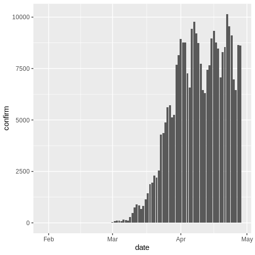
There are case data available for 489 days, but in an outbreak situation it is likely we would only have access to the beginning of this data set. Therefore we assume we only have the first 90 days of this data.
Delay distributions
We assume there are delays from the time of infection until the time a case is reported. We specify these delays as distributions to account for the uncertainty in individual level differences. The delay can consist of multiple types of delays/processes. A typical delay from time of infection to case reporting may consist of :
time from infection to symptom onset (the incubation period) + time from symptom onset to case notification (the reporting time) .
The delay distribution for each of these processes can either estimated from data or obtained from the literature. We can express uncertainty about what the correct parameters of the distributions by assuming the distributions have fixed parameters or whether they have variable parameters. To understand the difference between fixed and variable distributions, let’s consider the incubation period.
Delays and data
The number of delays and type of delay is a flexible input that depends on the data. The examples below highlight how the delays can be specified for different data sources:
| Data source | Delay(s) |
|---|---|
| Time of case report | Incubation period + time from symptom onset to case notification |
| Time of hospitalisation | Incubation period + time from symptom onset to hospitalisation |
| Time of symptom onset | Incubation period |
Incubation period distribution
The distribution of incubation period can usually be obtained from
the literature. The package {epiparameter} contains a
library of epidemiological parameters for different diseases obtained
from the literature.
We specify a (fixed) gamma distribution with mean \(\mu = 4\) and standard deviation \(\sigma^2= 2\) (shape = \(4\), scale = \(1\)) using the function
dist_spec() as follows:
R
incubation_period_fixed <- dist_spec(
  mean = 4, sd = 2,
  max = 20, distribution = "gamma"
)
incubation_period_fixed
OUTPUT
Fixed distribution with PMF [0.019 0.12 0.21 0.21 0.17 0.11 0.069 0.039 0.021 0.011 0.0054 0.0026 0.0012 0.00058 0.00026 0.00012 5.3e-05 2.3e-05 1e-05 4.3e-06]The argument max is the maximum value the distribution
can take, in this example 20 days.
Why a gamma distrubution?
The incubation period has to be positive in value. Therefore we must
specific a distribution in dist_spec which is for positive
values only.
dist_spec() supports log normal and gamma distributions,
which are distributions for positive values only.
For all types of delay, we will need to use distributions for positive values only - we don’t want to include delays of negative days in our analysis!
Including distribution uncertainty
To specify a variable distribution, we include uncertainty around the mean \(\mu\) and standard deviation \(\sigma^2\) of our gamma distribution. If our incubation period distribution has a mean \(\mu\) and standard deviation \(\sigma^2\), then we assume the mean (\(\mu\)) follows a Normal distribution with standard deviation \(\sigma_{\mu}^2\):
\[\mbox{Normal}(\mu,\sigma_{\mu}^2)\]
and a standard deviation (\(\sigma^2\)) follows a Normal distribution with standard deviation \(\sigma_{\sigma^2}^2\):
\[\mbox{Normal}(\sigma^2,\sigma_{\sigma^2}^2).\]
We specify this using dist_spec with the additional
arguments mean_sd (\(\sigma_{\mu}^2\)) and sd_sd
(\(\sigma_{\sigma^2}^2\)).
R
incubation_period_variable <- dist_spec(
  mean = 4, sd = 2,
  mean_sd = 0.5, sd_sd = 0.5,
  max = 20, distribution = "gamma"
)
incubation_period_variable
OUTPUT
Uncertain gamma distribution with (untruncated) mean 4 (SD 0.5) and SD 2 (SD 0.5)Reporting delays
After the incubation period, there will be an additional delay of time from symptom onset to case notification: the reporting delay. We can specify this as a fixed or variable distribution, or estimate a distribution from data.
When specifying a distribution, it is useful to visualise the
probability density to see the peak and spread of the distribution, in
this case we will use a log normal distribution. We can use the
functions convert_to_logmean() and
convert_to_logsd() to convert the mean and standard
deviation of a normal distribution to that of a log normal
distribution.
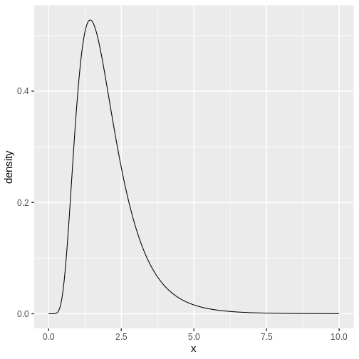
If we want to assume that the mean reporting delay is 2 days (with a standard deviation of 1 day), the log normal distribution will look like:
R
log_mean <- convert_to_logmean(2, 1)
log_sd <- convert_to_logsd(2, 1)
x <- seq(from = 0, to = 10, length = 1000)
df <- data.frame(x = x, density = dlnorm(x, meanlog = log_mean, sdlog = log_sd))
ggplot(df) +
  geom_line(
    aes(x, density)
  ) +
  theme_grey(
    base_size = 15
  )
Using the mean and standard deviation for the log normal
distribution, we can specify a fixed or variable distribution using
dist_spec() as before:
R
reporting_delay_variable <- dist_spec(
  mean = log_mean, sd = log_sd,
  mean_sd = 0.5, sd_sd = 0.5,
  max = 10, distribution = "lognormal"
)
If data is available on the time between symptom onset and reporting,
we can use the function estimate_delay() to estimate a log
normal distribution from a vector of delays. The code below illustrates
how to use estimate_delay() with synthetic delay data.
R
delay_data <- rlnorm(500, log(5), 1) # synthetic delay data
reporting_delay <- estimate_delay(
  delay_data,
  samples = 1000,
  bootstraps = 10
)
Generation time
We also must specify a distribution for the generation time. Here we will use a log normal distribution with mean 3.6 and standard deviation 3.1 (Ganyani et al. 2020).
R
generation_time_variable <- dist_spec(
  mean = 3.6, sd = 3.1,
  mean_sd = 0.5, sd_sd = 0.5,
  max = 20, distribution = "lognormal"
)
Finding estimates
The function epinow() is a wrapper for the function
estimate_infections() used to estimate cases by date of
infection. The generation time distribution and delay distributions must
be passed using the functions generation_time_opts() and
delay_opts() respectively.
There are numerous other inputs that can be passed to
epinow(), see EpiNow2::?epinow() for more
detail. One optional input is to specify a log normal prior for the
effective reproduction number \(R_t\)
at the start of the outbreak. We specify a mean and standard deviation
as arguments of prior within rt_opts():
R
rt_log_mean <- convert_to_logmean(2, 1)
rt_log_sd <- convert_to_logsd(2, 1)
rt <- rt_opts(prior = list(mean = rt_log_mean, sd = rt_log_sd))
Bayesian inference using Stan
The Bayesian inference is performed using MCMC methods with the
program Stan. There are a number of
default inputs to the Stan functions including the number of chains and
number of samples per chain (see
?EpiNow2::stan_opts()).
To reduce computation time, we can run chains in parallel. To do
this, we must set the number of cores to be used. By default, 4 MCMC
chains are run (see stan_opts()$chains), so we can set an
equal number of cores to be used in parallel as follows:
R
withr::local_options(list(mc.cores = 4))
To find the maximum number of available cores on your machine, use
parallel::detectCores().
Note : in the code below fixed distributions are used instead of variable. This is to speed up computation time. It is generally recommended to use variable distributions that account for additional uncertainty.
R
reported_cases <- cases[1:90, ]
estimates <- epinow(
  reported_cases = reported_cases,
  generation_time = generation_time_opts(generation_time_fixed),
  delays = delay_opts(incubation_period_fixed + reporting_delay_fixed),
  rt = rt_opts(prior = list(mean = rt_log_mean, sd = rt_log_sd))
)
OUTPUT
WARN [2024-09-24 01:23:52] epinow: There were 3 divergent transitions after warmup. See
https://mc-stan.org/misc/warnings.html#divergent-transitions-after-warmup
to find out why this is a problem and how to eliminate them. -
WARN [2024-09-24 01:23:52] epinow: Examine the pairs() plot to diagnose sampling problems
 -
Results
We can extract and visualise estimates of the effective reproduction number through time:
R
estimates$plots$R
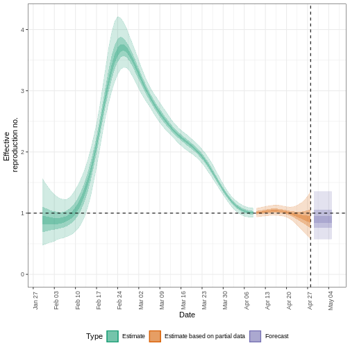
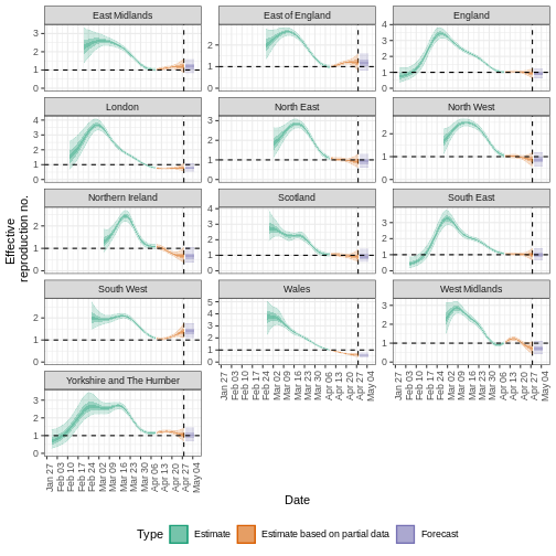
The uncertainty in the estimates increases through time. This is because estimates are informed by data in the past - within the delay periods. This difference in uncertainty is categorised into Estimate (green) utilises all data and Estimate based on partial data (orange) estimates that are based on less data (because infections that happened at the time are more likely to not have been observed yet) and therefore have increasingly wider intervals towards the date of the last data point. Finally, the Forecast (purple) is a projection ahead of time.
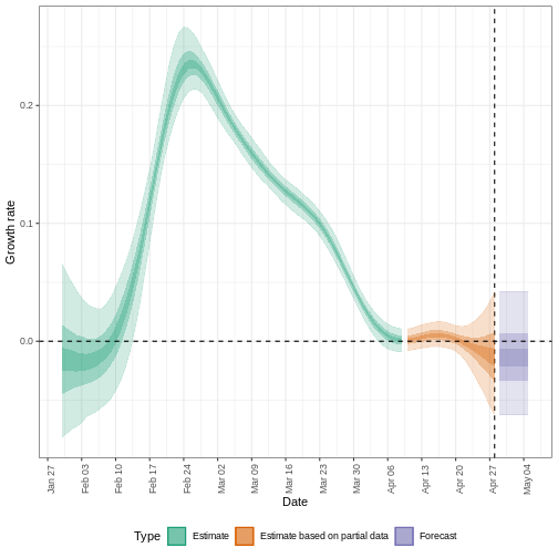
We can also visualise the growth rate estimate through time:
R
estimates$plots$growth_rate
To extract a summary of the key transmission metrics at the latest date in the data:
R
summary(estimates)
OUTPUT
                                 measure                 estimate
                                  <char>                   <char>
1: New confirmed cases by infection date     7267 (4048 -- 12834)
2:        Expected change in daily cases        Likely decreasing
3:            Effective reproduction no.        0.9 (0.58 -- 1.4)
4:                        Rate of growth -0.014 (-0.063 -- 0.042)
5:          Doubling/halving time (days)          -51 (16 -- -11)
As these estimates are based on partial data, they have a wide uncertainty interval.
From the summary of our analysis we see that the expected change in daily cases is Likely decreasing with the estimated new confirmed cases 7267 (4048 – 12834).
The effective reproduction number \(R_t\) estimate (on the last date of the data) is 0.9 (0.58 – 1.4).
The exponential growth rate of case numbers is -0.014 (-0.063 – 0.042).
The doubling time (the time taken for case numbers to double) is -51 (16 – -11).
Expected change in daily cases
A factor describing expected change in daily cases based on the posterior probability that \(R_t < 1\).
| Probability (\(p\)) | Expected change |
|---|---|
| \(p < 0.05\) | Increasing |
| \(0.05 \leq p< 0.4\) | Likely increasing |
| \(0.4 \leq p< 0.6\) | Stable |
| \(0.6 \leq p < 0.95\) | Likely decreasing |
| \(0.95 \leq p \leq 1\) | Decreasing |
Quantify geographical heterogeneity
The outbreak data of the start of the COVID-19 pandemic from the United Kingdom from the R package incidence2 includes the region in which the cases were recorded. To find regional estimates of the effective reproduction number and cases, we must format the data to have three columns:
-
date: the date, -
region: the region, -
confirm: number of confirmed cases for a region on a given date.
R
regional_cases <-
  incidence2::covidregionaldataUK[, c("date", "cases_new", "region")]
colnames(regional_cases) <- c("date", "confirm", "region")

# extract the first 90 dates for all regions
dates <- sort(unique(regional_cases$date))[1:90]
regional_cases <- regional_cases[which(regional_cases$date %in% dates), ]

head(regional_cases)
OUTPUT
        date confirm          region
1 2020-01-30      NA   East Midlands
2 2020-01-30      NA East of England
3 2020-01-30       2         England
4 2020-01-30      NA          London
5 2020-01-30      NA      North East
6 2020-01-30      NA      North West
To find regional estimates, we use the same inputs as
epinow() to the function
regional_epinow():
R
estimates_regional <- regional_epinow(
  reported_cases = regional_cases,
  generation_time = generation_time_opts(generation_time_fixed),
  delays = delay_opts(incubation_period_fixed + reporting_delay_fixed),
  rt = rt_opts(prior = list(mean = rt_log_mean, sd = rt_log_sd))
)
OUTPUT
INFO [2024-09-24 01:23:57] Producing following optional outputs: regions, summary, samples, plots, latest
INFO [2024-09-24 01:23:57] Reporting estimates using data up to: 2020-04-28
INFO [2024-09-24 01:23:57] No target directory specified so returning output
INFO [2024-09-24 01:23:57] Producing estimates for: East Midlands, East of England, England, London, North East, North West, Northern Ireland, Scotland, South East, South West, Wales, West Midlands, Yorkshire and The Humber
INFO [2024-09-24 01:23:57] Regions excluded: none
INFO [2024-09-24 02:07:37] Completed regional estimates
INFO [2024-09-24 02:07:37] Regions with estimates: 13
INFO [2024-09-24 02:07:37] Regions with runtime errors: 0
INFO [2024-09-24 02:07:37] Producing summary
INFO [2024-09-24 02:07:37] No summary directory specified so returning summary output
INFO [2024-09-24 02:07:38] No target directory specified so returning timings
R
estimates_regional$summary$summarised_results$table
OUTPUT
                      Region New confirmed cases by infection date
                      <char>                                <char>
 1:            East Midlands                      343 (213 -- 560)
 2:          East of England                      543 (331 -- 863)
 3:                  England                   3564 (2190 -- 5511)
 4:                   London                      293 (190 -- 452)
 5:               North East                      254 (147 -- 431)
 6:               North West                      557 (330 -- 877)
 7:         Northern Ireland                         43 (22 -- 84)
 8:                 Scotland                      283 (157 -- 539)
 9:               South East                      596 (354 -- 965)
10:               South West                      416 (293 -- 601)
11:                    Wales                        95 (64 -- 141)
12:            West Midlands                      270 (141 -- 486)
13: Yorkshire and The Humber                      481 (278 -- 784)
    Expected change in daily cases Effective reproduction no.
                            <fctr>                     <char>
 1:              Likely increasing          1.2 (0.85 -- 1.6)
 2:              Likely increasing          1.2 (0.83 -- 1.6)
 3:              Likely decreasing         0.91 (0.64 -- 1.2)
 4:              Likely decreasing         0.78 (0.56 -- 1.1)
 5:              Likely decreasing         0.91 (0.61 -- 1.3)
 6:              Likely decreasing         0.86 (0.58 -- 1.2)
 7:              Likely decreasing           0.64 (0.38 -- 1)
 8:              Likely decreasing          0.9 (0.58 -- 1.4)
 9:                         Stable         0.99 (0.67 -- 1.4)
10:                     Increasing           1.4 (1.1 -- 1.8)
11:                     Decreasing        0.57 (0.42 -- 0.77)
12:              Likely decreasing         0.71 (0.42 -- 1.1)
13:                         Stable            1 (0.69 -- 1.4)
                Rate of growth Doubling/halving time (days)
                        <char>                       <char>
 1:    0.023 (-0.021 -- 0.068)               30 (10 -- -33)
 2:    0.023 (-0.023 -- 0.067)               31 (10 -- -30)
 3:    -0.011 (-0.053 -- 0.03)              -61 (23 -- -13)
 4:   -0.03 (-0.066 -- 0.0098)              -23 (71 -- -11)
 5:   -0.011 (-0.057 -- 0.037)              -61 (19 -- -12)
 6:   -0.019 (-0.062 -- 0.023)              -37 (30 -- -11)
 7:    -0.052 (-0.1 -- 0.0053)            -13 (130 -- -6.8)
 8:   -0.013 (-0.062 -- 0.047)              -53 (15 -- -11)
 9: -0.00095 (-0.047 -- 0.046)             -730 (15 -- -15)
10:     0.046 (0.013 -- 0.084)               15 (8.3 -- 54)
11:  -0.065 (-0.094 -- -0.032)            -11 (-21 -- -7.4)
12:   -0.041 (-0.092 -- 0.012)             -17 (59 -- -7.5)
13:   0.0033 (-0.044 -- 0.051)              210 (14 -- -16)
R
estimates_regional$summary$plots$R
Summary
EpiNow2 can be used to estimate transmission metrics
from case data at the start of an outbreak. The reliability of these
estimates depends on the quality of the data and appropriate choice of
delay distributions. In the next tutorial we will learn how to make
forecasts and investigate some of the additional inference options
available in EpiNow2.
Key Points
- Transmission metrics can be estimated from case data after accounting for delays
- Uncertainty can be accounted for in delay distributions
