Projecting re-emergence risk after waning or new births

If population immunity accumulates during an epidemic, then the peak of the epidemic is the point at which there is a sufficient reduction in susceptibility to bring the effective reproduction number \(R\) below the critical value of 1. However, because infections continue as the epidemic declines, more immunity can accumulate, and hence \(R\) can be substantially below 1 at the end of the epidemic.

New to finalsize? We’d recommend the “Get started” and “Modelling uncertainty in R₀” vignettes first!

Use case

We want to know long it might take for a (partially) immunising infection to re-emerge following an initial large epidemic. This question has been common for emerging vector-borne infections like Zika and Chikungunya (Kucharski et al. 2016).

What we have

1. In addition to the \(R_0\), data on waning of immunity and population birth rates.
2. A measure of the error in the estimated \(R_0\) of the infection.

What we assume

1. An SIR epidemic, assuming everyone fully susceptible initially and mixing is random. This simplifying assumption has previously been used for modelling emerging vector-borne infections like Zika (Andronico et al. 2017).

2. Gradual waning of immunity, with a certain proportion of immune individuals becoming susceptible again each year. Note: we can set this proportion equal to zero for a no-waning scenario.

3. Gradual influx of new susceptibles via an annual birth rate (which is equal to the death rate so the population size remains constant).

Code

# load finalsize
library(finalsize)
library(ggplot2)

Modelling the initial epidemic

We follow the approach described in the “Modelling uncertainty in R₀” vignette, which includes uncertainty in final size calculations by running final_size() for values drawn from a distribution, and summarising the outcomes.

For simplicity, here we use a model that assumes a uniformly mixing population. A similar approach could be used for multiple age groups, although this would require more assumptions about waning of age specific susceptibility and population turnover to ensure consistent demographic patterns.

First we define the future window of time we are considering, as well as the rate of waning (assumed to be 5% per year) and influx of new susceptibles (assuming 14 births per 1,000 per year).

We also define a distribution of \(R_0\) values for the initial epidemic and the second later re-emerging outbreak, both following a normal distribution \(N(\mu = 2, \sigma = 0.3)\).

Code

# future time period considered
years_range <- seq(0, 20)

# proportion losing immunity per year
annual_wane <- 0.05

# proportion newly susceptible per year
birth_rate <- 14 / 1000

# define r0 values
r0_mean <- 2.0
r0_samples <- rnorm(n = 100, mean = r0_mean, sd = 0.3) # for first outbreak
r0_samples2 <- rnorm(n = 100, mean = r0_mean, sd = 0.3) # for second outbreak

Next we simulate initial epidemics using final_size(), iterating over \(R_0\) values sampled above.

Code

# run final size for each value and collate estimates
# use `Map()` to iterate over values and an index to add to the final data
final_size_est <- Map(
  function(r0, i) {
    fs <- final_size(r0)$p_infected # run final size model, get estimate only
    data.frame(fs = fs, i = i, r0 = r0) # data.frame for each value considered
  },
  r0 = r0_samples,
  i = seq_along(r0_samples)
)

# use Reduce to combine the list of data.frames into a single data.frame
final_size_df <- Reduce(rbind, final_size_est)

Modelling waning immunity and influx of susceptibles

We calculate the relative population immunity, accounting for the waning of immunity from the initial epidemic, and accounting for the influx (due to new births) of new susceptibles over a range of 20 years.

This is calculated as \(I_y = (1 - \text{annual waning})^y \times (1 - b y)\), where \(b\) is the birth rate; this is vectorised over the range of years in the code.

Code

# define changes in susceptibility over time from waning
# and population turnover (assuming) rectangular age distribution
relative_immunity <- (1 - annual_wane)^(years_range) *
  pmax(1 - birth_rate * years_range, 0) # use pmax in case of longer year range

Projected estimates of effective \(R\)

Having simulated the distribution of initial epidemic sizes based on the distribution of \(R_0\), we next implement waning and an influx of new susceptibles to calculate the level of immunity over coming years, relative to the level of immunity at the end of the epidemic. This is a step-wise process:

• The initial final size calculations have given us estimates of the population’s ‘relative immunity’ in year 0 (i.e., the final size; assuming all recovered individuals are immune);

• This allows us to calculate the relative susceptibility from the relative immunity, as \(\text{susceptibility} = 1 - I_y\); this can be calculated for any year \(y\) using the predicted immunity for that year \(I_y\);

• The effective reproduction number (i.e. \(R\) for a partially susceptible population) can then be calculated as \(R = R_0 \times \text{susceptibility}\) for each year;

• We can then predict \(R\) over the coming years as population susceptibility increases.

When \(R\) rises above the critical value of 1, there is potential for sustained transmission in the population and hence another large epidemic.

We calculate the level of susceptibility - and hence \(R\) - over the distribution of \(R_0\) values we have assumed for a re-emerging epidemic.

In this example, the distribution is the same as the original epidemic (which is plausible if it is the same pathogen and setting), but we could alter this assumption if we think factors like population density or climate change might change the transmissibility of the infection in future.

Code

# calculate effective R for each value and collate estimates
r_eff_est <- Map(
  function(r0, fs) {
    r_eff <- (1 - fs * relative_immunity) * r0

    # data.frame for each value considered
    data.frame(r_eff = r_eff, yr = years_range)
  },
  r0 = r0_samples2,
  fs = final_size_df$fs
)

# use Reduce to combine the list of data.frames into a single data.frame
r_eff_df <- Reduce(rbind, r_eff_est)

In this scenario, the majority of new susceptibility comes from waning, rather than influx of new births (i.e. 5% vs 1.4% per year). As a result, the predicted value of \(R\) rises substantially in the years following the initial epidemic, suggesting potential for re-emergence within 5-10 years.

Code

# plot results
ggplot(r_eff_df) +
  geom_hline(yintercept = 1, linetype = "dashed", color = "gray") +
  geom_vline(xintercept = 0, colour = "red", linetype = "dashed") +
  annotate(
    geom = "text",
    x = 0, y = 2, angle = 90, vjust = "outward",
    colour = "red",
    label = "Initial epidemic at year 0"
  ) +
  stat_summary(
    aes(
      yr, r_eff
    ),
    fun = mean,
    fun.min = function(x) {
      quantile(x, 0.025)
    },
    fun.max = function(x) {
      quantile(x, 0.975)
    }
  ) +
  scale_y_continuous(
    limits = c(0, 3)
  ) +
  theme_classic() +
  coord_cartesian(
    expand = TRUE
  ) +
  labs(
    x = "Years after initial epidemic",
    y = "Effective R (mean and 95% CI)"
  )

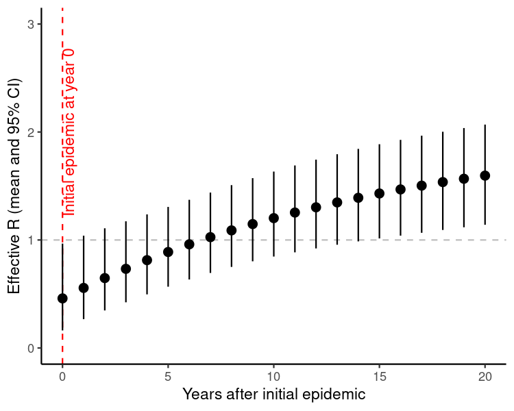
Figure 1: Predicted value of the effective reproduction number \(R\) following an initial epidemic of an emerging infection in year 0. We assume 5% of the immune population becomes susceptible again each year following the epidemic, and there is an influx of new susceptibles via a birth rate of 14/1000 per year. We also assume \(R_0\) has a mean of 2, with a standard deviation around this estimate of 0.3.

References

Andronico, Alessio, Frédérique Dorléans, Jean-Louis Fergé, Henrik Salje, Frédéric Ghawché, Aissatou Signate, Elise Daudens-Vaysse, et al. 2017. “Real-Time Assessment of Health-Care Requirements During the Zika Virus Epidemic in Martinique.” American Journal of Epidemiology 186 (10): 1194–1203. https://doi.org/10.1093/aje/kwx008.

Kucharski, Adam J., Sebastian Funk, Rosalind M. Eggo, Henri-Pierre Mallet, W. John Edmunds, and Eric J. Nilles. 2016. “Transmission Dynamics of Zika Virus in Island Populations: A Modelling Analysis of the 2013–14 French Polynesia Outbreak.” PLOS Neglected Tropical Diseases 10 (5): e0004726. https://doi.org/10.1371/journal.pntd.0004726.