Access epidemiological delay distributions

Last updated on 2024-05-04 | Edit this page

Overview

Questions

How to get access to disease delay distributions from a pre-established database for use in analysis?

Objectives

Get delays from a literature search database with {epiparameter}.
Get distribution parameters and summary statistics of delay distributions.

Prerequisites

This episode requires you to be familiar with:

Data science : Basic programming with R.

Epidemic theory : epidemiological parameters, disease time periods, such as the incubation period, generation time, and serial interval.

Introduction

Infectious diseases follow an infection cycle, which usually includes the following phases: presymptomatic period, symptomatic period and recovery period, as described by their natural history. These time periods can be used to understand transmission dynamics and inform disease prevention and control interventions.

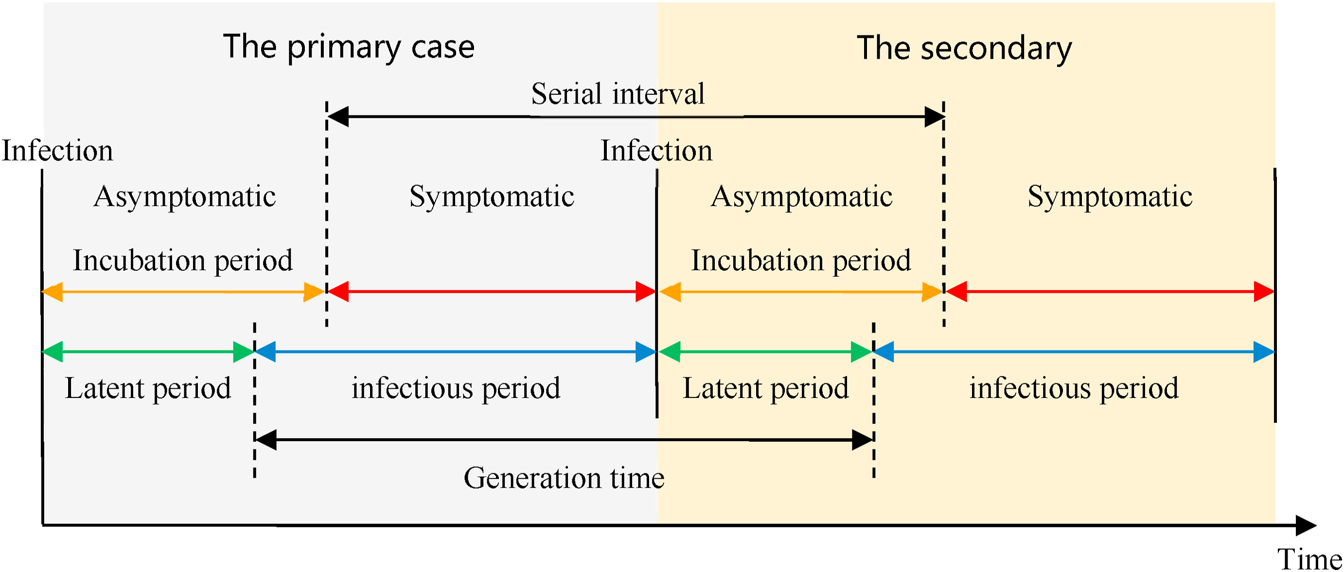
Definition of key time periods. From Xiang et al, 2021

Definitions

Look at the glossary for the definitions of all the time periods of the figure above!

However, early in an epidemic, modelling efforts can be delayed by the lack of a centralised resource that summarises input parameters for the disease of interest (Nash et al., 2023). Projects like {epiparameter} and {epireview} are building online catalogues following literature synthesis protocols that can help parametrise models by easily accessing a comprenhensive library of previously estimated epidemiological parameters from past outbreaks.

To exemplify how to use the {epiparameter} R package in your analysis pipeline, our goal in this episode will be to choose one specific set of epidemiological parameters from the literature, instead of copying-and-pasting them by hand, to plug them into an EpiNow2 analysis workflow.

Let’s start loading the {epiparameter} package. We’ll use the pipe %>% to connect some of their functions, some tibble and dplyr functions, so let’s also call to the tidyverse package:

R

library(epiparameter)
library(tidyverse)

The problem

If we want to estimate the transmissibility of an infection, it’s common to use a package such as EpiEstim or EpiNow2. However, both require some epidemiological information as an input. For example, in EpiNow2 we use EpiNow2::dist_spec() to specify a generation time as a probability distribution adding its mean, standard deviation (sd), and maximum value (max). To specify a generation_time that follows a Gamma distribution with mean $\mu = 4$, standard deviation $\sigma = 2$, and a maximum value of 20, we write:

R

generation_time <- 
  EpiNow2::dist_spec(
    mean = 4,
    sd = 2,
    max = 20,
    distribution = "gamma"
  )

It is a common practice for analysts to manually search the available literature and copy and paste the summary statistics or the distribution parameters from scientific publications. A challenge that is often faced is that the reporting of different statistical distributions is not consistent across the literature. {epiparameter}’s objective is to facilitate the access to reliable estimates of distribution parameters for a range of infectious diseases, so that they can easily be implemented in outbreak analytic pipelines.

In this episode, we will choose the summary statistics from the library of epidemiological parameters provided by {epiparameter}.

Generation time vs serial interval

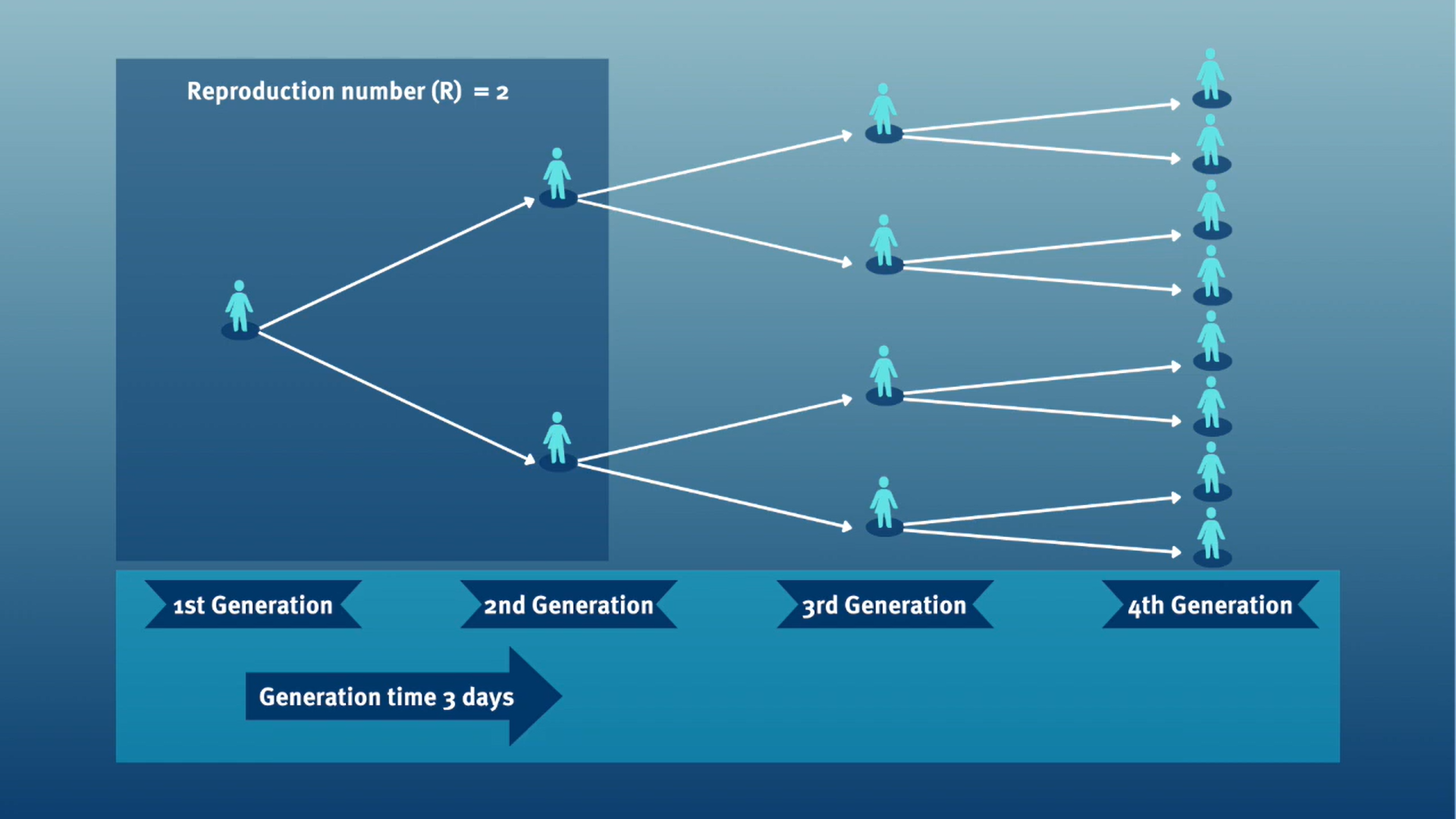
The generation time, jointly with the reproduction number ($R$), provide valuable insights on the strength of transmission and inform the implementation of control measures. Given a $R>1$, the shorter the generation time, the earlier the incidence of disease cases will grow.

Video from the MRC Centre for Global Infectious Disease Analysis, Ep 76. Science In Context - Epi Parameter Review Group with Dr Anne Cori (27-07-2023) at https://youtu.be/VvpYHhFDIjI?si=XiUyjmSV1gKNdrrL

In calculating the effective reproduction number ($R_{t}$), the generation time distribution is often approximated by the serial interval distribution. This frequent approximation is because it is easier to observe and measure the onset of symptoms than the onset of infectiousness.

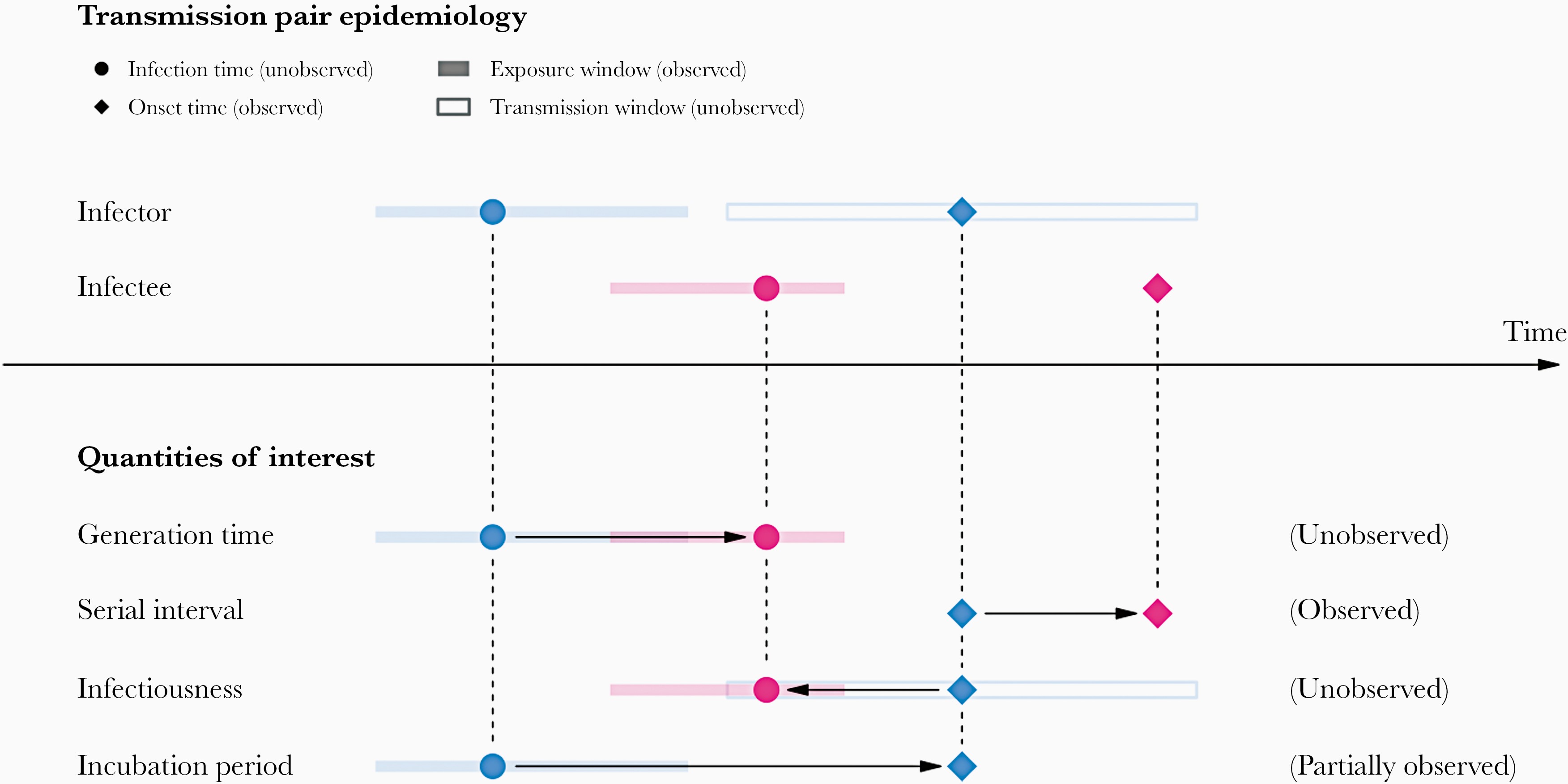
A schematic of the relationship of different time periods of transmission between an infector and an infectee in a transmission pair. Exposure window is defined as the time interval having viral exposure, and transmission window is defined as the time interval for onward transmission with respect to the infection time (Chung Lau et al., 2021).

However, using the serial interval as an approximation of the generation time is primarily valid for diseases in which infectiousness starts after symptom onset (Chung Lau et al., 2021). In cases where infectiousness starts before symptom onset, the serial intervals can have negative values, which is the case for diseases with pre-symptomatic transmission (Nishiura et al., 2020).

From time periods to probability distributions.

When we calculate the serial interval, we see that not all case pairs have the same time length. We will observe this variability for any case pair and individual time period, including the incubation period and infectious period.

Serial intervals of possible case pairs in (a) COVID-19 and (b) MERS-CoV. Pairs represent a presumed infector and their presumed infectee plotted by date of symptom onset (Althobaity et al., 2022).

To summarise these data from individual and pair time periods, we can find the statistical distributions that best fit the data (McFarland et al., 2023).

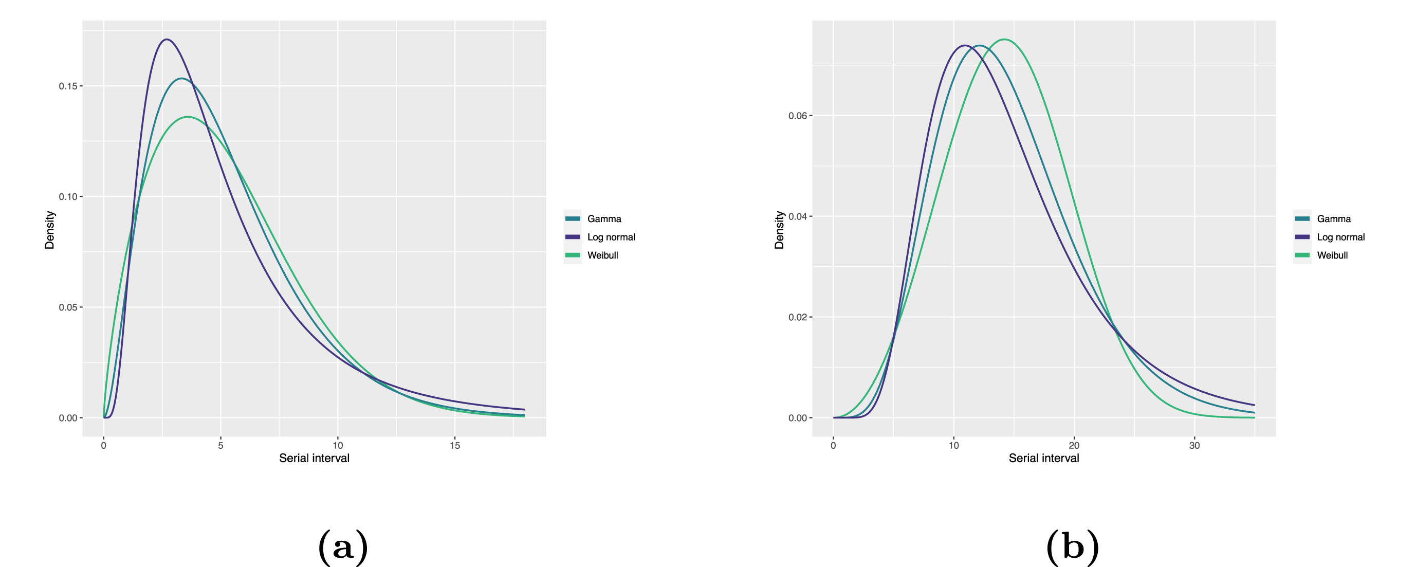
Fitted serial interval distribution for (a) COVID-19 and (b) MERS-CoV based on reported transmission pairs in Saudi Arabia. We fitted three commonly used distributions, Lognormal, Gamma, and Weibull distributions, respectively (Althobaity et al., 2022).

Statistical distributions are summarised in terms of their summary statistics like the location (mean and percentiles) and spread (variance or standard deviation) of the distribution, or with their distribution parameters that inform about the form (shape and rate/scale) of the distribution. These estimated values can be reported with their uncertainty (95% confidence intervals).

Gamma	mean	shape	rate/scale
MERS-CoV	14.13(13.9–14.7)	6.31(4.88–8.52)	0.43(0.33–0.60)
COVID-19	5.1(5.0–5.5)	2.77(2.09–3.88)	0.53(0.38–0.76)

Weibull	mean	shape	rate/scale
MERS-CoV	14.2(13.3–15.2)	3.07(2.64–3.63)	16.1(15.0–17.1)
COVID-19	5.2(4.6–5.9)	1.74(1.46–2.11)	5.83(5.08–6.67)

Serial interval estimates using Gamma, Weibull, and Log normal distributions. 95% confidence intervals for the shape and scale (logmean and sd for Log normal) parameters are shown in brackets (Althobaity et al., 2022).
Log normal	mean	mean-log	sd-log
MERS-CoV	14.08(13.1–15.2)	2.58(2.50–2.68)	0.44(0.39–0.5)
COVID-19	5.2(4.2–6.5)	1.45(1.31–1.61)	0.63(0.54–0.74)

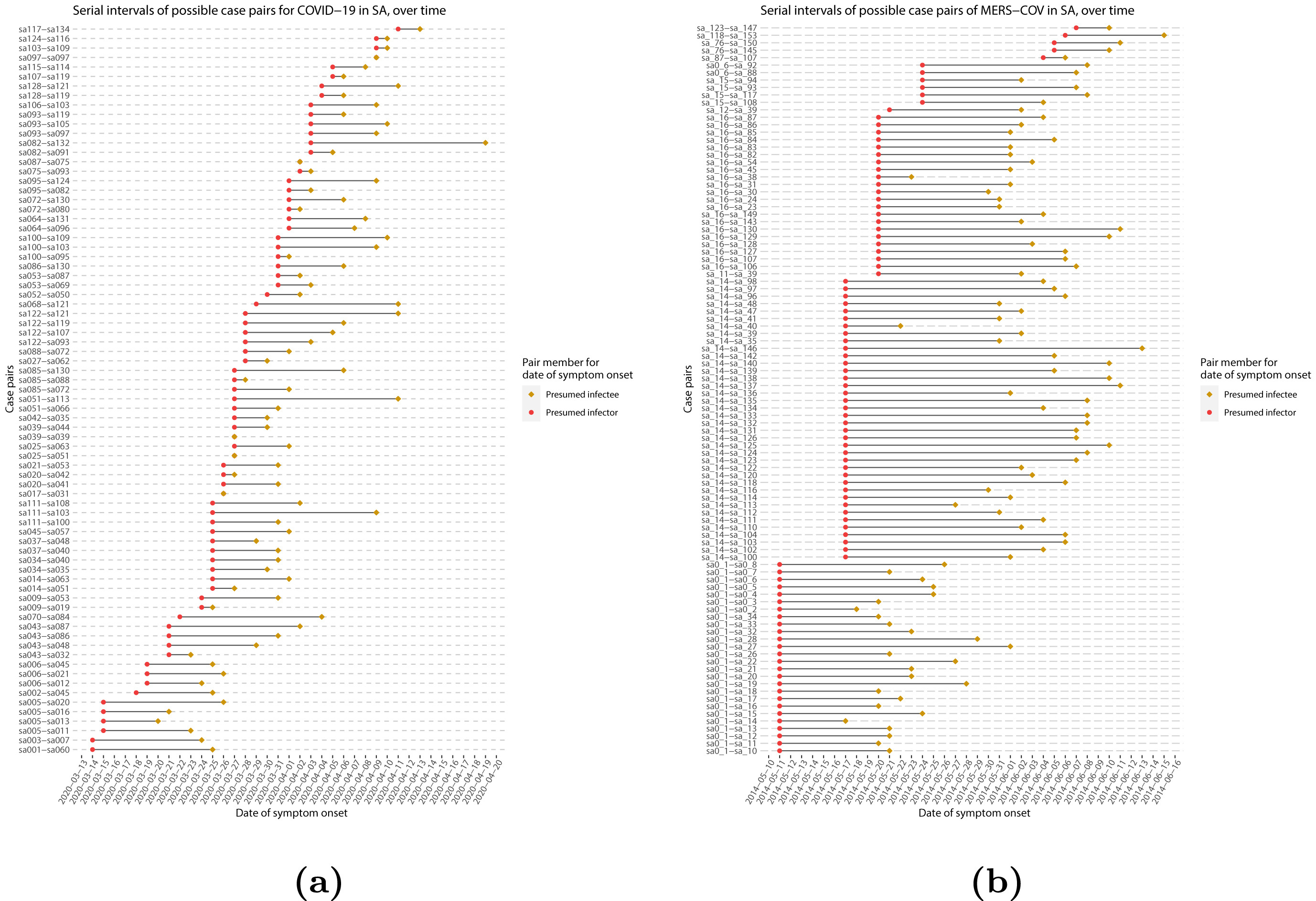
Serial interval

Assume that COVID-19 and SARS have similar reproduction number values and that the serial interval approximates the generation time.

Given the Serial interval of both infections in the figure below:

Which one would be harder to control?
Why do you conclude that?

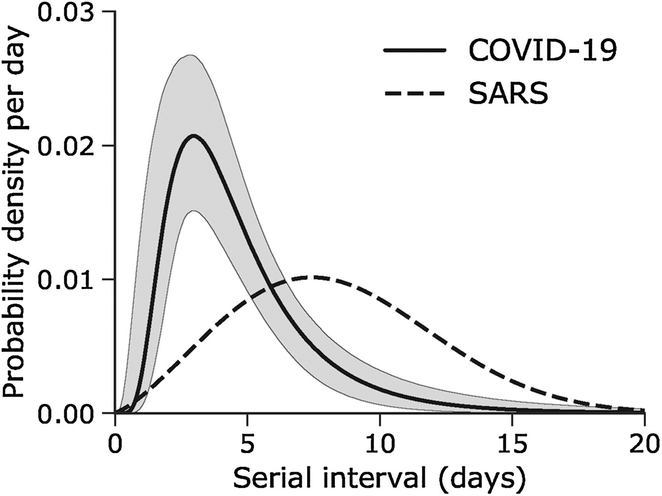
Serial interval of novel coronavirus (COVID-19) infections overlaid with a published distribution of SARS. (Nishiura et al., 2020)

Give me a hint

The peak of each curve can inform you about the location of the mean of each distribution. The larger the mean, the larger the serial interval.

Show me the solution

Which one would be harder to control?

COVID-19

Why do you conclude that?

COVID-19 has the lowest mean serial interval. The approximate mean value for the serial interval of COVID-19 is around four days, and SARS is about seven days. Thus, COVID-19 will likely have newer generations in less time than SARS, assuming similar reproduction numbers.

Choosing epidemiological parameters

In this section, we will use {epiparameter} to obtain the generation time and the serial interval for COVID-19, so these metrics can be used to estimate the transmissibility of this disease using EpiNow2 in subsequent sections of this episode.

Let’s start by looking at how many entries are available in the epidemiological distributions database in {epiparameter} (epidist_db) for the disease named covid-19:

R

epiparameter::epidist_db(
  disease = "covid"
)

OUTPUT

Returning 27 results that match the criteria (22 are parameterised). 
Use subset to filter by entry variables or single_epidist to return a single entry. 
To retrieve the short citation for each use the 'get_citation' function

OUTPUT

List of <epidist> objects
  Number of entries in library: 27
  Number of studies in library: 10
  Number of diseases: 1
  Number of delay distributions: 27
  Number of offspring distributions: 0

The double-colon

The double-colon :: in R is used to access functions or objects from a specific package without loading the entire package into the current environment. This allows for a more targeted approach to using package components and helps avoid namespace conflicts.

:: lets you call a specific function from a package by explicitly mentioning the package name. For example, dplyr::filter(data, condition) uses filter() from the dplyr package without loading the entire package.

From the {epiparameter} package, we can use the epidist_db() function to ask for any disease and also for a specific epidemiological distribution (epi_dist).

Let’s ask now how many parameters we have in the epidemiological distributions database (epidist_db) with the generation time using the string generation:

R

epiparameter::epidist_db(
  epi_dist = "generation"
)

OUTPUT

Returning 1 results that match the criteria (1 are parameterised). 
Use subset to filter by entry variables or single_epidist to return a single entry. 
To retrieve the short citation for each use the 'get_citation' function

OUTPUT

Disease: Influenza
Pathogen: Influenza-A-H1N1
Epi Distribution: generation time
Study: Lessler J, Reich N, Cummings D, New York City Department of Health and
Mental Hygiene Swine Influenza Investigation Team (2009). "Outbreak of
2009 Pandemic Influenza A (H1N1) at a New York City School." _The New
England Journal of Medicine_. doi:10.1056/NEJMoa0906089
<https://doi.org/10.1056/NEJMoa0906089>.
Distribution: weibull
Parameters:
  shape: 2.360
  scale: 3.180

Currently, in the library of epidemiological parameters, we have one generation time entry for Influenza. Considering the above-mentioned considerations, we can look at the serial intervals for COVID-19. Run this locally!

R

epiparameter::epidist_db(
  disease = "COVID",
  epi_dist = "serial"
)

With this query combination, we get more than one delay distribution. This output is an <epidist> class object.

CASE-INSENSITIVE

epidist_db is case-insensitive. This means that you can use strings with letters in upper or lower case indistinctly. Strings like "serial", "serial interval" or "serial_interval" are also valid.

To summarise an <epidist> object and get the column names from the underlying parameter database, we can add the epiparameter::list_distributions() function to the previous code using the pipe %>%:

R

epiparameter::epidist_db(
  disease = "covid",
  epi_dist = "serial"
) %>%
  epiparameter::list_distributions()

OUTPUT

Returning 4 results that match the criteria (3 are parameterised). 
Use subset to filter by entry variables or single_epidist to return a single entry. 
To retrieve the short citation for each use the 'get_citation' function

OUTPUT

   disease epi_distribution prob_distribution       author year
1 COVID-19  serial interval              <NA> Muluneh .... 2021
2 COVID-19  serial interval             lnorm Hiroshi .... 2020
3 COVID-19  serial interval           weibull Hiroshi .... 2020
4 COVID-19  serial interval              norm Lin Yang.... 2020

In the epiparameter::list_distributions() output, we can also find different types of probability distributions (e.g., Log-normal, Weibull, Normal).

{epiparameter} uses the base R naming convention for distributions. This is why Lognormal is called lnorm.

Why do we have a ‘NA’ entry?

Entries with a missing value (<NA>) in the prob_distribution column are non-parameterised entries. They have summary statistics but no probability distribution. Compare these two outputs:

R

# get an <epidist> object
distribution <-
  epiparameter::epidist_db(
    disease = "covid",
    epi_dist = "serial"
  )

distribution %>%
  # pluck the first entry in the object class <list>
  pluck(1) %>%
  # check if <epidist> object have distribution parameters
  is_parameterised()

# check if the second <epidist> object
# have distribution parameters
distribution %>%
  pluck(2) %>%
  is_parameterised()

Parameterised entries have an Inference method

As detailed in ?is_parameterised, a parameterised distribution is the entry that has a probability distribution associated with it provided by an inference_method as shown in metadata:

R

distribution[[1]]$metadata$inference_method
distribution[[2]]$metadata$inference_method
distribution[[4]]$metadata$inference_method

Find your delay distributions!

Take 2 minutes to explore the {epiparameter} library.

Choose a disease of interest (e.g., Influenza, Measles, etc.) and a delay distribution (e.g., the incubation period, onset to death, etc.).

Find:

How many delay distributions are for that disease?
How many types of probability distribution (e.g., gamma, lognormal) are for a given delay in that disease?

Ask:

Do you recognise the papers?
Should {epiparameter} literature review consider any other paper?

Give me a hint

The epidist_db() function with disease alone counts the number of entries like:

studies, and
delay distributions.

The epidist_db() function with disease and epi_dist gets a list of all entries with:

the complete citation,
the type of a probability distribution, and
distribution parameter values.

The combo of epidist_db() plus list_distributions() gets a data frame of all entries with columns like:

the type of the probability distribution per delay, and
author and year of the study.

Show me the solution

We choose to explore Ebola’s delay distributions:

R

# we expect 16 delays distributions for ebola
epiparameter::epidist_db(
  disease = "ebola"
)

OUTPUT

Returning 17 results that match the criteria (17 are parameterised). 
Use subset to filter by entry variables or single_epidist to return a single entry. 
To retrieve the short citation for each use the 'get_citation' function

OUTPUT

List of <epidist> objects
  Number of entries in library: 17
  Number of studies in library: 4
  Number of diseases: 1
  Number of delay distributions: 16
  Number of offspring distributions: 1

Now, from the output of epiparameter::epidist_db(), What is an offspring distribution?

We choose to find Ebola’s incubation periods. This output list all the papers and parameters found. Run this locally if needed:

R

epiparameter::epidist_db(
  disease = "ebola",
  epi_dist = "incubation"
)

We use list_distributions() to get a summary display of all:

R

# we expect 2 different types of delay distributions
# for ebola incubation period
epiparameter::epidist_db(
  disease = "ebola",
  epi_dist = "incubation"
) %>%
  list_distributions()

OUTPUT

Returning 5 results that match the criteria (5 are parameterised). 
Use subset to filter by entry variables or single_epidist to return a single entry. 
To retrieve the short citation for each use the 'get_citation' function

OUTPUT

              disease  epi_distribution prob_distribution       author year
1 Ebola Virus Disease incubation period             lnorm Martin E.... 2011
2 Ebola Virus Disease incubation period             gamma WHO Ebol.... 2015
3 Ebola Virus Disease incubation period             gamma WHO Ebol.... 2015
4 Ebola Virus Disease incubation period             gamma WHO Ebol.... 2015
5 Ebola Virus Disease incubation period             gamma WHO Ebol.... 2015

We find two types of probability distributions for this query: lognormal and gamma.

How does {epiparameter} do the collection and review of peer-reviewed literature? We invite you to read the vignette on “Data Collation and Synthesis Protocol”!

Select a single distribution

The epiparameter::epidist_db() function works as a filtering or subset function. Let’s use the author argument to filter Hiroshi Nishiura parameters:

R

epiparameter::epidist_db(
  disease = "covid",
  epi_dist = "serial",
  author = "Hiroshi"
) %>%
  epiparameter::list_distributions()

OUTPUT

Returning 2 results that match the criteria (2 are parameterised). 
Use subset to filter by entry variables or single_epidist to return a single entry. 
To retrieve the short citation for each use the 'get_citation' function

OUTPUT

   disease epi_distribution prob_distribution       author year
1 COVID-19  serial interval             lnorm Hiroshi .... 2020
2 COVID-19  serial interval           weibull Hiroshi .... 2020

We still get more than one epidemiological parameter. We can set the single_epidist argument to TRUE to only one:

R

epiparameter::epidist_db(
  disease = "covid",
  epi_dist = "serial",
  author = "Hiroshi",
  single_epidist = TRUE
)

OUTPUT

Using Nishiura H, Linton N, Akhmetzhanov A (2020). "Serial interval of novel
coronavirus (COVID-19) infections." _International Journal of
Infectious Diseases_. doi:10.1016/j.ijid.2020.02.060
<https://doi.org/10.1016/j.ijid.2020.02.060>.. 
To retrieve the short citation use the 'get_citation' function

OUTPUT

Disease: COVID-19
Pathogen: SARS-CoV-2
Epi Distribution: serial interval
Study: Nishiura H, Linton N, Akhmetzhanov A (2020). "Serial interval of novel
coronavirus (COVID-19) infections." _International Journal of
Infectious Diseases_. doi:10.1016/j.ijid.2020.02.060
<https://doi.org/10.1016/j.ijid.2020.02.060>.
Distribution: lnorm
Parameters:
  meanlog: 1.386
  sdlog: 0.568

How does ‘single_epidist’ works?

Looking at the help documentation for ?epiparameter::epidist_db():

If multiple entries match the arguments supplied and single_epidist = TRUE, then the parameterised <epidist> with the largest sample size will be returned.
If multiple entries are equal after this sorting, the first entry will be returned.

What is a parametrised <epidist>? Look at ?is_parameterised.

Let’s assign this <epidist> class object to the covid_serialint object.

R

covid_serialint <-
  epiparameter::epidist_db(
    disease = "covid",
    epi_dist = "serial",
    author = "Nishiura",
    single_epidist = TRUE
  )

You can use plot() to <epidist> objects to visualise:

the Probability Density Function (PDF) and
the Cumulative Distribution Function (CDF).

R

# plot <epidist> object
plot(covid_serialint)

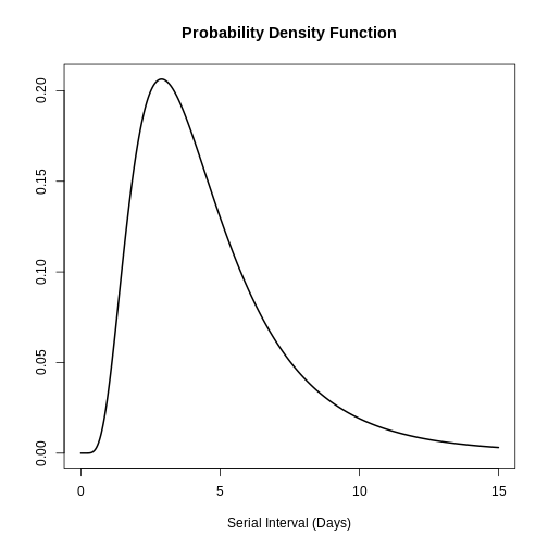
With the day_range argument, you can change the length or number of days in the x axis. Explore what this looks like:

R

# plot <epidist> object
plot(covid_serialint, day_range = 0:20)

Extract the summary statistics

We can get the mean and standard deviation (sd) from this <epidist> diving into the summary_stats object:

R

# get the mean
covid_serialint$summary_stats$mean

OUTPUT

[1] 4.7

Now, we have an epidemiological parameter we can reuse! We can replace the summary statistics numbers we plug into the EpiNow2::dist_spec() function:

R

generation_time <- 
  EpiNow2::dist_spec(
    mean = covid_serialint$summary_stats$mean, # replaced!
    sd = covid_serialint$summary_stats$sd, # replaced!
    max = 20,
    distribution = "gamma"
  )

In the next episode we’ll learn how to use EpiNow2 to correctly specify distributions, estimate transmissibility. Then, how to use distribution functions to get a maximum value (max) for EpiNow2::dist_spec() and use {epiparameter} in your analysis.

Log normal distributions

If you need the log normal distribution parameters instead of the summary statistics, we can use epiparameter::get_parameters():

R

covid_serialint_parameters <-
  epiparameter::get_parameters(covid_serialint)

covid_serialint_parameters

OUTPUT

  meanlog     sdlog 
1.3862617 0.5679803

This gets a vector of class <numeric> ready to use as input for any other package!

Challenges

Ebola’s serial interval

Take 1 minute to:

Get access to the Ebola serial interval with the highest sample size.

Answer:

What is the sd of the epidemiological distribution?
What is the sample_size used in that study?

Give me a hint

Use the $ operator plus the tab or ↹ keyboard button to explore them as an expandable list:

R

covid_serialint$

Use the str() to display the structure of the <epidist> R object.

Show me the solution

R

# ebola serial interval
ebola_serial <-
  epiparameter::epidist_db(
    disease = "ebola",
    epi_dist = "serial",
    single_epidist = TRUE
  )

OUTPUT

Using WHO Ebola Response Team, Agua-Agum J, Ariyarajah A, Aylward B, Blake I,
Brennan R, Cori A, Donnelly C, Dorigatti I, Dye C, Eckmanns T, Ferguson
N, Formenty P, Fraser C, Garcia E, Garske T, Hinsley W, Holmes D,
Hugonnet S, Iyengar S, Jombart T, Krishnan R, Meijers S, Mills H,
Mohamed Y, Nedjati-Gilani G, Newton E, Nouvellet P, Pelletier L,
Perkins D, Riley S, Sagrado M, Schnitzler J, Schumacher D, Shah A, Van
Kerkhove M, Varsaneux O, Kannangarage N (2015). "West African Ebola
Epidemic after One Year — Slowing but Not Yet under Control." _The New
England Journal of Medicine_. doi:10.1056/NEJMc1414992
<https://doi.org/10.1056/NEJMc1414992>.. 
To retrieve the short citation use the 'get_citation' function

R

ebola_serial

OUTPUT

Disease: Ebola Virus Disease
Pathogen: Ebola Virus
Epi Distribution: serial interval
Study: WHO Ebola Response Team, Agua-Agum J, Ariyarajah A, Aylward B, Blake I,
Brennan R, Cori A, Donnelly C, Dorigatti I, Dye C, Eckmanns T, Ferguson
N, Formenty P, Fraser C, Garcia E, Garske T, Hinsley W, Holmes D,
Hugonnet S, Iyengar S, Jombart T, Krishnan R, Meijers S, Mills H,
Mohamed Y, Nedjati-Gilani G, Newton E, Nouvellet P, Pelletier L,
Perkins D, Riley S, Sagrado M, Schnitzler J, Schumacher D, Shah A, Van
Kerkhove M, Varsaneux O, Kannangarage N (2015). "West African Ebola
Epidemic after One Year — Slowing but Not Yet under Control." _The New
England Journal of Medicine_. doi:10.1056/NEJMc1414992
<https://doi.org/10.1056/NEJMc1414992>.
Distribution: gamma
Parameters:
  shape: 2.188
  scale: 6.490

R

# get the sd
ebola_serial$summary_stats$sd

OUTPUT

[1] 9.6

R

# get the sample_size
ebola_serial$metadata$sample_size

OUTPUT

[1] 305

Try to visualise this distribution using plot().

Also, explore all the other nested elements within the <epidist> object.

Share about:

What elements do you find useful for your analysis?
What other elements would you like to see in this object? How?

Ebola’s severity parameter

A severity parameter like the duration of hospitalisation could add to the information needed about the bed capacity in response to an outbreak (Cori et al., 2017).

For Ebola:

What is the reported point estimate of the mean duration of health care and case isolation?

Give me a hint

An informative delay should measure the time from symptom onset to recovery or death.

Find a way to access the whole {epiparameter} database and find how that delay may be stored. The list_distributions() output is a dataframe.

Show me the solution

R

# one way to get the list of all the available parameters
epidist_db(disease = "all") %>%
  list_distributions() %>%
  as_tibble() %>%
  distinct(epi_distribution)

OUTPUT

Returning 122 results that match the criteria (99 are parameterised). 
Use subset to filter by entry variables or single_epidist to return a single entry. 
To retrieve the short citation for each use the 'get_citation' function

OUTPUT

# A tibble: 12 × 1
   epi_distribution            
   <chr>                       
 1 incubation period           
 2 serial interval             
 3 generation time             
 4 onset to death              
 5 offspring distribution      
 6 hospitalisation to death    
 7 hospitalisation to discharge
 8 notification to death       
 9 notification to discharge   
10 onset to discharge          
11 onset to hospitalisation    
12 onset to ventilation

R

ebola_severity <- epidist_db(
  disease = "ebola",
  epi_dist = "onset to discharge"
)

OUTPUT

Returning 1 results that match the criteria (1 are parameterised). 
Use subset to filter by entry variables or single_epidist to return a single entry. 
To retrieve the short citation for each use the 'get_citation' function

R

# point estimate
ebola_severity$summary_stats$mean

OUTPUT

[1] 15.1

Check that for some {epiparameter} entries you will also have the uncertainty around the point estimate of each summary statistic:

R

# 95% confidence intervals
ebola_severity$summary_stats$mean_ci

OUTPUT

[1] 95

R

# limits of the confidence intervals
ebola_severity$summary_stats$mean_ci_limits

OUTPUT

[1] 14.6 15.6

The distribution Zoo

Explore this shinyapp called The Distribution Zoo!

Follow these steps to reproduce the form of the COVID serial interval distribution from {epiparameter} (covid_serialint object):

Access the https://ben18785.shinyapps.io/distribution-zoo/ shiny app website,
Go to the left panel,
Keep the Category of distribution: Continuous Univariate,
Select a new Type of distribution: Log-Normal,
Move the sliders, i.e. the graphical control element that allows you to adjust a value by moving a handle along a horizontal track or bar to the covid_serialint parameters.

Replicate these with the distribution object and all its list elements: [[2]], [[3]], and [[4]]. Explore how the shape of a distribution changes when its parameters change.

Share about:

What other features of the website do you find helpful?

Key Points

Use {epiparameter} to access the literature catalogue of epidemiological delay distributions.
Use epidist_db() to select single delay distributions.
Use list_distributions() for an overview of multiple delay distributions.
Reuse known estimates for unknown disease in the early stage of an outbreak when no contact tracing data is available.