Use delay distributions in analysis
Last updated on 2026-07-04 | Edit this page
Overview
Questions
- How to reuse delays stored in the epiparameter library with my existing analysis pipeline?
Objectives
- Use distribution functions with continuous and discrete
distributions stored as
<epiparameter>objects. - Convert a continuous to a discrete distribution with epiparameter.
- Connect epiparameter outputs with EpiNow2 inputs.
Prerequisites
- Complete tutorial Access epidemiological delay distributions
- Complete tutorial Quantifying transmission
This episode requires you to be familiar with:
Data science : Basic programming with R.
Statistics : Probability distributions.
Epidemic theory : Epidemiological parameters, time periods, Effective reproductive number.
Introduction
This episode will integrate the content of the two previous episodes.
Let’s start by loading the epiparameter and
EpiNow2 package. We’ll use the pipe %>%,
some dplyr verbs and ggplot2, so let’s
also call to the tidyverse package:
R
library(epiparameter)
library(EpiNow2)
library(tidyverse)
To recap, we learned that epiparameter helps us to choose one specific set of epidemiological parameters from the literature, instead of copy/pasting them by hand:
R
covid_serialint <-
  epiparameter::epiparameter_db(
    disease = "covid",
    epi_name = "serial",
    single_epiparameter = TRUE
  )
Now, we have an epidemiological parameter that we can use in our
analysis! However, we can’t use this object directly for
analysis. For example, to quantify transmission, we often use the serial
interval distribution as an approximation of the generation time. To do
this we need to apply additional functions to an
<epiparameter> object to extract its summary
statistics or distribution parameters. These
outputs can then be used as inputs for EpiNow2::LogNormal()
or EpiNow2::Gamma(), just as we did in the previous
episode.
In this episode, we will use the distribution
functions that epiparameter provides to get
descriptive values like the median, maximum value (max),
percentiles, or quantiles. This set of functions can operate on
any distribution that can be included in an
<epiparameter> object: Gamma, Weibull, Lognormal,
Negative Binomial, Geometric, and Poisson, which are mostly used in
outbreak analytics.
You’ll need these outputs in the next episodes to power your analysis pipelines — so let’s make sure you’re comfortable working with them before moving on!
The double-colon
The double-colon :: in R lets you call a specific
function from a package without loading the entire package into the
current environment.
For example, dplyr::filter(data, condition) uses
filter() from the dplyr package.
This helps us remember package functions and avoid namespace conflicts by explicitly specifying which package’s function to use when multiple packages have functions with the same name.
Distribution functions
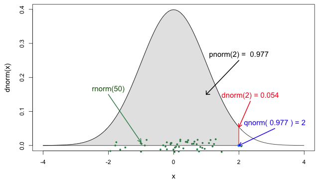
In R, all the statistical distributions have functions to access the following:
-
density(): Probability Density function (PDF), -
cdf(): Cumulative Distribution function (CDF), -
quantile(): Quantile function, and -
generate(): Random values from the given distribution.
Functions for the Normal distribution
If you need it, read in detail about the R probability functions for the normal distribution, each of its definitions and identify in which part of a distribution they are located!
If you look at ?stats::Distributions, each type of
distribution has a unique set of functions. However,
epiparameter gives you the same four functions to access
each of the values above for any <epiparameter>
object you want!
R
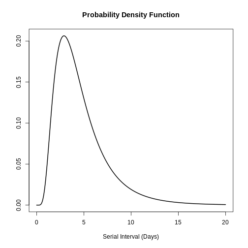
# plot this to have a visual reference

# continuous distribution
plot(covid_serialint, xlim = c(0, 20))
R
# the density value at quantile value of 10 (days)
density(covid_serialint, at = 10)
OUTPUT
[1] 0.01911607R
# the cumulative probability at quantile value of 10 (days)
epiparameter::cdf(covid_serialint, q = 10)
OUTPUT
[1] 0.9466605R
# the quantile value (day) at a cumulative probability of 60%
quantile(covid_serialint, p = 0.6)
OUTPUT
[1] 4.618906R
# generate 10 random values (days) given
# the distribution family and its parameters
epiparameter::generate(covid_serialint, times = 10)
OUTPUT
 [1]  4.022843  6.177242  2.579687 17.801526  3.680146  4.829783  4.659798
[8] 3.263045 2.205161 1.414135Window for contact tracing and the serial interval
The serial interval is important in the optimisation of contact tracing since it provides a time window for the containment of a disease spread (Fine, 2003). Depending on the serial interval, we can evaluate the need to increase the number of days considered for contact tracing to include more backwards contacts (Davis et al., 2020).
With the COVID-19 serial interval (covid_serialint)
calculate:
- How much would expanding the contact tracing window from 2 to 6 days before symptom onset improve the detection of potential infectors?
The serial interval is the time between symptom onset in an infector and symptom onset in their infectee.
We can use the serial interval distribution to quantify the probability of detecting an infector from a new case. This probability can be calculated directly from the assumed distribution. Refer to Figure 2 in Davis et al., 2020.
For an object class <epiparameter>, the cumulative
probability can be computed using epiparameter::cdf().
R
plot(covid_serialint)
R
# calculate probability of finding backward cases
# with contact tracing window of 2 days
window_2 <- epiparameter::cdf(covid_serialint, q = 2)

window_2
OUTPUT
[1] 0.1111729R
# calculate probability of finding backward cases
# with contact tracing window of 6 days
window_6 <- epiparameter::cdf(covid_serialint, q = 6)

window_6
OUTPUT
[1] 0.7623645R
# calculate the difference
window_6 - window_2
OUTPUT
[1] 0.6511917Given the COVID-19 serial interval:
A contact tracing method considering contacts up to 2 days pre-onset will capture around 11.1% of backward cases.
If this period is extended to 6 days pre-onset, this could include 76.2% of backward contacts.
About 65.1% more backward cases could be captured when extending tracing from 2 to 6 days.
If we exchange the question between days and cumulative probability to:
- When considering secondary cases, within how many days following the symptom onset of primary cases can we expect 55% of secondary symptom onset to occur?
R
quantile(covid_serialint, p = 0.55)
An interpretation could be:
- 55% of secondary cases will have their symptom onset within around 4.3 days of symptom onset in the primary case.
Discretise a continuous distribution
We are getting closer to the end! EpiNow2::LogNormal()
still needs a maximum value (max).
One way to do this is to get the quantile value for the
distribution’s 99th percentile or 0.99 cumulative
probability. For this, we need access to the set of distribution
functions for our <epiparameter> object.
We can use the set of distribution functions for a
continuous distribution (as above). However, these values will
be continuous numbers. We can discretise the
continuous distribution stored in our <epiparameter>
object to get discrete values from a continuous distribution.
When we epiparameter::discretise() the continuous
distribution we get a discrete distribution:
R
covid_serialint_discrete <-
  epiparameter::discretise(covid_serialint)

covid_serialint_discrete
OUTPUT
Disease: COVID-19
Pathogen: SARS-CoV-2
Epi Parameter: serial interval
Study: Nishiura H, Linton N, Akhmetzhanov A (2020). "Serial interval of novel
coronavirus (COVID-19) infections." _International Journal of
Infectious Diseases_. doi:10.1016/j.ijid.2020.02.060
<https://doi.org/10.1016/j.ijid.2020.02.060>.
Distribution: discrete lnorm (days)
Parameters:
  meanlog: 1.386
  sdlog: 0.568
We identify this change in the Distribution: output line
of the <epiparameter> object. Double check this
line:
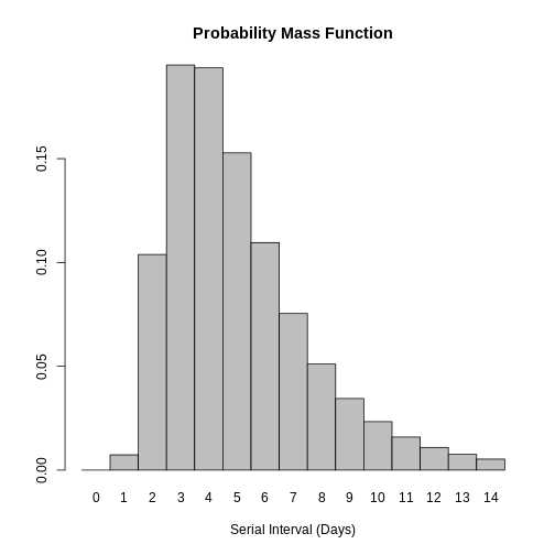
Distribution: discrete lnorm (days)While for a continuous distribution, we plot the Probability Density Function (PDF), for a discrete distribution, we plot the Probability Mass Function (PMF):
R
# discrete distribution
plot(covid_serialint_discrete)
To finally get a max value, let’s access the quantile
value of the 99th percentile or 0.99 cumulative probability
of the distribution using the quantile() function, as we
did above for the continuous distribution.
R
covid_serialint_discrete_max <-
  quantile(covid_serialint_discrete, p = 0.99)
Length of quarantine and incubation period
The incubation period distribution is a useful delay to assess the length of active monitoring or quarantine (Lauer et al., 2020). Similarly, delays from symptom onset to recovery (or death) will determine the required duration of health care and case isolation (Cori et al., 2017).
The library of parameters in the package epiparameter contains the parameters reported by Lauer et al., 2020.
Calculate:
- How many days after infection do 99% of people who will develop COVID-19 symptoms actually show symptoms? Get an integer as a response.
What delay distribution measures the time between infection and the onset of symptoms? For a refresher, you can read the tutorial Glossary.
The probability functions for <epiparameter>
discrete distributions are the same that we used for
the continuous ones!
R
# the delay from infection to onset is called incubation period
# access the incubation period for covid
covid_incubation <-
  epiparameter::epiparameter_db(
    disease = "covid",
    epi_name = "incubation",
    author = "lauer",
    single_epiparameter = TRUE
  )

covid_incubation
OUTPUT
Disease: COVID-19
Pathogen: SARS-CoV-2
Epi Parameter: incubation period
Study: Lauer S, Grantz K, Bi Q, Jones F, Zheng Q, Meredith H, Azman A, Reich
N, Lessler J (2020). "The Incubation Period of Coronavirus Disease 2019
(COVID-19) From Publicly Reported Confirmed Cases: Estimation and
Application." _Annals of Internal Medicine_. doi:10.7326/M20-0504
<https://doi.org/10.7326/M20-0504>.
Distribution: lnorm (days)
Parameters:
  meanlog: 1.629
  sdlog: 0.419
R
# to get an integer as a response, discretise the distribution
covid_incubation_discrete <- epiparameter::discretise(covid_incubation)

covid_incubation_discrete
OUTPUT
Disease: COVID-19
Pathogen: SARS-CoV-2
Epi Parameter: incubation period
Study: Lauer S, Grantz K, Bi Q, Jones F, Zheng Q, Meredith H, Azman A, Reich
N, Lessler J (2020). "The Incubation Period of Coronavirus Disease 2019
(COVID-19) From Publicly Reported Confirmed Cases: Estimation and
Application." _Annals of Internal Medicine_. doi:10.7326/M20-0504
<https://doi.org/10.7326/M20-0504>.
Distribution: discrete lnorm (days)
Parameters:
  meanlog: 1.629
  sdlog: 0.419
R
# calculate the quantile or value at the 99th percentile from the distribution
quantile(covid_incubation_discrete, p = 0.99)
OUTPUT
[1] 1399% of those who develop COVID-19 symptoms will do so within 13 days of infection.
Now, is this result consistent with the duration of quarantine recommended in practice during the COVID-19 pandemic?
Plug-in {epiparameter} to {EpiNow2}
Now we can plug everything into the EpiNow2::LogNormal()
function!
- the summary statistics
meanandsdof the distribution, - a maximum value
max, - the
distributionname.
When using EpiNow2::LogNormal() to define a log
normal distribution like the one in the
covid_serialint object we can specify the mean and sd as
parameters. Alternatively, to get the “natural” parameters for a log
normal distribution we can convert its summary statistics to
distribution parameters named meanlog and
sdlog. With epiparameter we can directly get
the distribution parameters using
epiparameter::get_parameters():
R
covid_serialint_parameters <-
  epiparameter::get_parameters(covid_serialint)
Then, we have:
R
serial_interval_covid <-
  EpiNow2::LogNormal(
    meanlog = covid_serialint_parameters["meanlog"],
    sdlog = covid_serialint_parameters["sdlog"],
    max = covid_serialint_discrete_max
  )

serial_interval_covid
OUTPUT
- lognormal distribution (max: 14):
  meanlog:
    1.4
  sdlog:
0.57LogNormal or Gamma?
Let’s say that you need to quantify the transmission of an Ebola outbreak. You will use the serial interval as an approximation of the generation time for EpiNow2. The epiparameter will give you access to the parameter estimated from historical outbreaks.
Follow these steps:
- Get access to the
serial intervaldistribution ofEbolausing epiparameter. - Access one entry from the study with the highest sample size.
- Print the output and read the description.
- Identify which probability distribution (e.g., Gamma, Lognormal, etc.) was used by the authors to model the delay.
- Extract the distribution parameters for the corresponding probability distribution.
- Calculate an exact maximum value for the delay distribution (e.g., the 99th percentile).
- Plug-in the distribution parameters from the
<epiparameter>to the corresponding probability distribution function in EpiNow2 (e.g.,EpiNow2::Gamma(),EpiNow2::LogNormal(), etc.).
When connecting epiparameter and EpiNow2, there is one step that is susceptible to mistakes.
In <epiparameter>, the output line
Distribution: determines the function to use from
EpiNow2:
We choose EpiNow2::Gamma() if in
<epiparameter> we get:
Distribution: gamma (days)
Parameters:
  shape: 2.188
  scale: 6.490
We choose EpiNow2::LogNormal() if in
<epiparameter> we get:
Distribution: lnorm (days)
Parameters:
  meanlog: 1.386
sdlog: 0.568R
# 1. access a serial interval
ebola_serialint <- epiparameter::epiparameter_db(
  disease = "ebola",
  epi_name = "serial",
  single_epiparameter = TRUE
)
R
ebola_serialint
OUTPUT
Disease: Ebola Virus Disease
Pathogen: Ebola Virus
Epi Parameter: serial interval
Study: WHO Ebola Response Team, Agua-Agum J, Ariyarajah A, Aylward B, Blake I,
Brennan R, Cori A, Donnelly C, Dorigatti I, Dye C, Eckmanns T, Ferguson
N, Formenty P, Fraser C, Garcia E, Garske T, Hinsley W, Holmes D,
Hugonnet S, Iyengar S, Jombart T, Krishnan R, Meijers S, Mills H,
Mohamed Y, Nedjati-Gilani G, Newton E, Nouvellet P, Pelletier L,
Perkins D, Riley S, Sagrado M, Schnitzler J, Schumacher D, Shah A, Van
Kerkhove M, Varsaneux O, Kannangarage N (2015). "West African Ebola
Epidemic after One Year — Slowing but Not Yet under Control." _The New
England Journal of Medicine_. doi:10.1056/NEJMc1414992
<https://doi.org/10.1056/NEJMc1414992>.
Distribution: gamma (days)
Parameters:
  shape: 2.188
  scale: 6.490
R
# 2. extract parameters from {epiparameter} object
ebola_serialint_params <- epiparameter::get_parameters(ebola_serialint)

ebola_serialint_params
OUTPUT
   shape    scale
2.187934 6.490141
R
# 3. get a maximum value
ebola_serialint_max <- ebola_serialint %>%
  epiparameter::discretise() %>%
  quantile(p = 0.99)

ebola_serialint_max
OUTPUT
[1] 45R
# 4. adapt {epiparameter} to the {EpiNow2} distribution interface
ebola_generationtime <- EpiNow2::Gamma(
  shape = ebola_serialint_params["shape"],
  scale = ebola_serialint_params["scale"],
  max = ebola_serialint_max
)

ebola_generationtime
OUTPUT
- gamma distribution (max: 45):
  shape:
    2.2
  rate:
    0.15
R
# plot the `epiparameter` class object
plot(ebola_serialint)
R
# plot the `dist_spec` class object from {EpiNow2}
plot(ebola_generationtime)
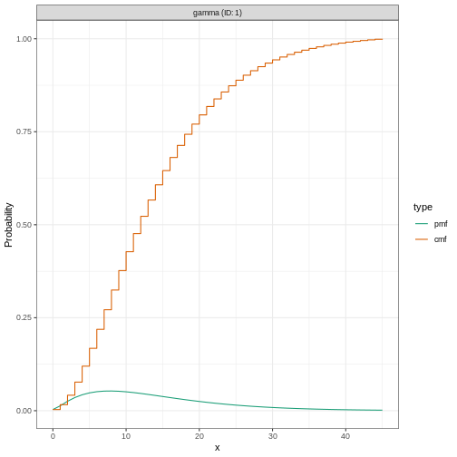
Plotting distributions from the EpiNow2 interface
always gives a discretised output. From the legend: PMF
stands for Probability Mass Function and CMF stands for
Cumulative Mass Function.
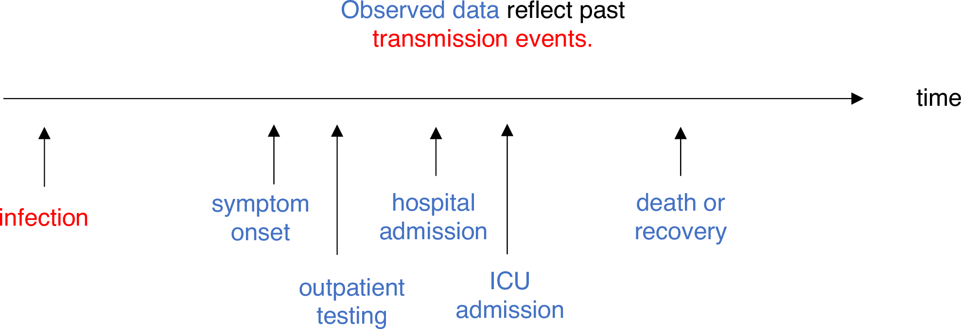
Adjusting for reporting delays
Estimating \(R_t\) requires data on the daily number of new infections. Due to lags in the development of detectable viral loads, symptom onset, seeking care, and reporting, these numbers are not readily available. All observations reflect transmission events from some time in the past. In other words, if \(d\) is the delay from infection to observation, then observations at time \(t\) inform \(R_{t−d}\), not \(R_t\). (Gostic et al., 2020)
The delay distribution could be inferred jointly
with the underlying times of infection or estimated as the sum of the incubation period distribution and
the distribution of delays from symptom onset to observation from line
list data (reporting delay).
For EpiNow2, we can specify these two complementary delay
distributions in the delays argument.
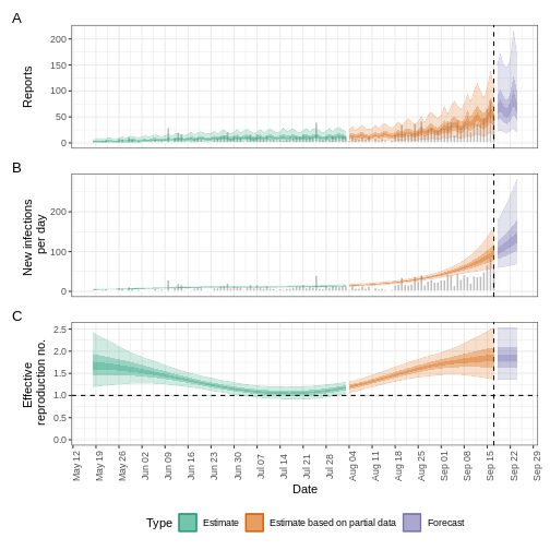
Use an incubation period for COVID-19 to estimate Rt
Estimate the time-varying reproduction number for the first 60 days
of the example_confirmed data set from
EpiNow2. Access to an incubation period for COVID-19 from
epiparameter to use it as a reporting delay.
Use the last epinow() calculation using the
delays argument and the delay_opts() helper
function.
The delays argument and the delay_opts()
helper function are analogous to the generation_time
argument and the generation_time_opts() helper
function.
R
epinow_estimates <- EpiNow2::epinow(
  # cases
  data = example_confirmed[1:60],
  # delays
  generation_time = EpiNow2::generation_time_opts(covid_serial_interval),
  delays = EpiNow2::delay_opts(covid_incubation_time)
)
R
# generation time ---------------------------------------------------------
# get covid serial interval
covid_serialint <-
epiparameter::epiparameter_db(
disease = "covid",
epi_name = "serial",
single_epiparameter = TRUE
)
# adapt epiparameter to epinow2
covid_serialint_discrete_max <- covid_serialint %>%
epiparameter::discretise() %>%
quantile(p = 0.99)
covid_serialint_parameters <-
epiparameter::get_parameters(covid_serialint)
covid_serial_interval <-
EpiNow2::LogNormal(
meanlog = covid_serialint_parameters["meanlog"],
sdlog = covid_serialint_parameters["sdlog"],
max = covid_serialint_discrete_max
)
# incubation time ---------------------------------------------------------
# get covid incubation period
covid_incubation <- epiparameter::epiparameter_db(
disease = "covid",
epi_name = "incubation",
single_epiparameter = TRUE
)
# adapt epiparameter to epinow2
covid_incubation_discrete_max <- covid_incubation %>%
epiparameter::discretise() %>%
quantile(p = 0.99)
covid_incubation_parameters <-
epiparameter::get_parameters(covid_incubation)
covid_incubation_time <-
EpiNow2::LogNormal(
meanlog = covid_incubation_parameters["meanlog"],
sdlog = covid_incubation_parameters["sdlog"],
max = covid_incubation_discrete_max
)
# epinow ------------------------------------------------------------------
# Set 4 cores to be used in parallel computations
withr::local_options(list(mc.cores = parallel::detectCores() - 1))
# run epinow
epinow_estimates_cgi <- EpiNow2::epinow(
# cases
data = example_confirmed[1:60],
# delays
generation_time = EpiNow2::generation_time_opts(covid_serial_interval),
delays = EpiNow2::delay_opts(covid_incubation_time)
)
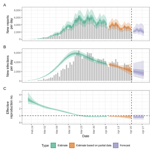
base::plot(epinow_estimates_cgi)
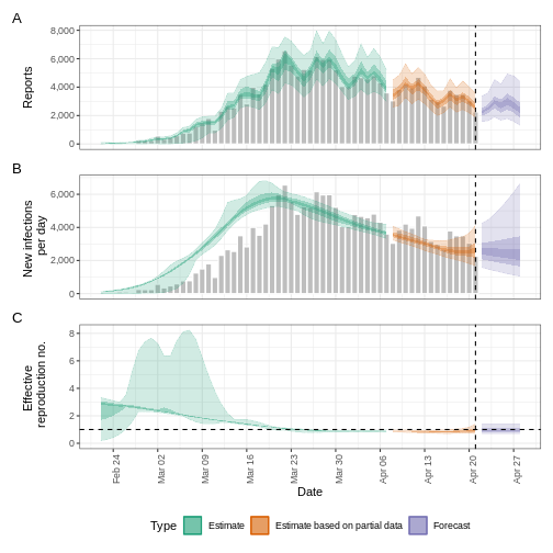
Try to complement the delays argument with a reporting
delay like the reporting_delay_fixed object of the previous
episode.
How much has it changed?
Compare three runs of EpiNow2::epinow():
- Use only the generation time
- Add the incubation time
- Add the incubation time and reporting delay
After adding all delays, discuss:
- Does the trend of the model fit in the “Estimate” section change?
- Has the uncertainty changed?
- How would you explain or interpret any of these changes?
Compare all the EpiNow2 figures generated in the three runs.
Challenges
A code completion tip
If we write the [] next to the object
covid_serialint_parameters[], within [] we can
use the Tab key ↹ for code
completion feature
This gives quick access to
covid_serialint_parameters["meanlog"] and
covid_serialint_parameters["sdlog"].
We invite you to try this out in code chunks and the R console!
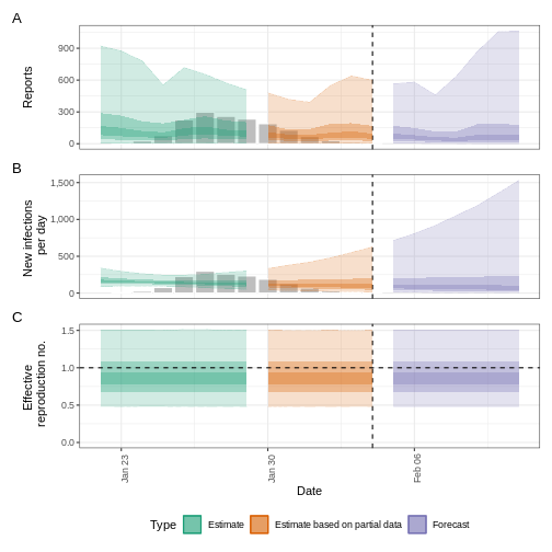
Ebola’s effective reproduction number adjusted by reporting delays
Download and read the Ebola dataset:
- Estimate the effective reproduction number using EpiNow2
- Adjust the estimate by the available reporting delays in epiparameter
- Why did you choose that parameter?
To calculate the \(R_t\) using EpiNow2, we need:
- Aggregated incidence
data, with confirmed cases per day, and - The
generationtime distribution. - Optionally, reporting
delaysdistributions when available (e.g., incubation period).
To get delay distribution using epiparameter we can use functions like:
epiparameter::epiparameter_db()epiparameter::parameter_tbl()discretise()quantile()
R
# read data
# e.g.: if path to file is data/raw-data/ebola_cases.csv then:
ebola_confirmed <-
  read_csv(here::here("data", "raw-data", "ebola_cases.csv")) %>%
  incidence2::incidence(
    date_index = "date",
    counts = "confirm",
    count_values_to = "confirm",
    date_names_to = "date",
    complete_dates = TRUE
  ) %>%
  dplyr::select(-count_variable)

# list distributions
epiparameter::epiparameter_db(disease = "ebola") %>%
  epiparameter::parameter_tbl()
R
# generation time ---------------------------------------------------------

# subset one distribution for the generation time
ebola_serial <- epiparameter::epiparameter_db(
  disease = "ebola",
  epi_name = "serial",
  single_epiparameter = TRUE
)

# adapt epiparameter to epinow2
ebola_serial_discrete <- epiparameter::discretise(ebola_serial)

serial_interval_ebola <-
  EpiNow2::Gamma(
    mean = ebola_serial$summary_stats$mean,
    sd = ebola_serial$summary_stats$sd,
    max = quantile(ebola_serial_discrete, p = 0.99)
  )

# incubation time ---------------------------------------------------------

# subset one distribution for delay of the incubation period
ebola_incubation <- epiparameter::epiparameter_db(
  disease = "ebola",
  epi_name = "incubation",
  single_epiparameter = TRUE
)

# adapt epiparameter to epinow2
ebola_incubation_discrete <- epiparameter::discretise(ebola_incubation)

incubation_period_ebola <-
  EpiNow2::Gamma(
    mean = ebola_incubation$summary_stats$mean,
    sd = ebola_incubation$summary_stats$sd,
    max = quantile(ebola_incubation_discrete, p = 0.99)
  )

# epinow ------------------------------------------------------------------

# run epinow
epinow_estimates_egi <- EpiNow2::epinow(
  # cases
  data = ebola_confirmed,
  # delays
  generation_time = EpiNow2::generation_time_opts(serial_interval_ebola),
  delays = EpiNow2::delay_opts(incubation_period_ebola)
)

plot(epinow_estimates_egi)
What to do with Weibull distributions?
Use the influenza_england_1978_school dataset from the
outbreaks package to calculate the effective reproduction
number using EpiNow2 adjusting by the available reporting
delays in epiparameter.
EpiNow2::NonParametric() accepts Probability Mass
Functions (PMF) from any distribution family. Read the reference guide
on Probability
distributions.
R
# What parameters are available for Influenza?
epiparameter::epiparameter_db(disease = "influenza") %>%
  epiparameter::parameter_tbl() %>%
  count(epi_name)
OUTPUT
# Parameter table:
# A data frame:    3 × 2
  epi_name              n
  <chr>             <int>
1 generation time       1
2 incubation period    15
3 serial interval       1
R
# generation time ---------------------------------------------------------

# Read the generation time
influenza_generation <-
  epiparameter::epiparameter_db(
    disease = "influenza",
    epi_name = "generation"
  )

influenza_generation
OUTPUT
Disease: Influenza
Pathogen: Influenza-A-H1N1
Epi Parameter: generation time
Study: Lessler J, Reich N, Cummings D, New York City Department of Health and
Mental Hygiene Swine Influenza Investigation Team (2009). "Outbreak of
2009 Pandemic Influenza A (H1N1) at a New York City School." _The New
England Journal of Medicine_. doi:10.1056/NEJMoa0906089
<https://doi.org/10.1056/NEJMoa0906089>.
Distribution: weibull (days)
Parameters:
  shape: 2.360
  scale: 3.180
R
# EpiNow2 currently accepts Gamma or LogNormal
# other can pass the PMF function

influenza_generation_discrete <-
  epiparameter::discretise(influenza_generation)

influenza_generation_max <-
  quantile(influenza_generation_discrete, p = 0.99)

influenza_generation_pmf <-
  density(
    influenza_generation_discrete,
    at = 0:influenza_generation_max
  )

influenza_generation_pmf
OUTPUT
[1] 0.00000000 0.06312336 0.22134988 0.29721220 0.23896828 0.12485164 0.04309454R
# EpiNow2::NonParametric() can also accept the PMF values
generation_time_influenza <-
  EpiNow2::NonParametric(
    pmf = influenza_generation_pmf
  )

# incubation period -------------------------------------------------------

# Read the incubation period
influenza_incubation <-
  epiparameter::epiparameter_db(
    disease = "influenza",
    epi_name = "incubation",
    single_epiparameter = TRUE
  )

# Discretise incubation period
influenza_incubation_discrete <-
  epiparameter::discretise(influenza_incubation)

influenza_incubation_max <-
  quantile(influenza_incubation_discrete, p = 0.99)

influenza_incubation_pmf <-
  density(
    influenza_incubation_discrete,
    at = 0:influenza_incubation_max
  )

influenza_incubation_pmf
OUTPUT
[1] 0.00000000 0.05749151 0.16687705 0.22443092 0.21507632 0.16104546 0.09746609
[8] 0.04841928
R
# EpiNow2::NonParametric() can also accept the PMF values
incubation_time_influenza <-
  EpiNow2::NonParametric(
    pmf = influenza_incubation_pmf
  )

# epinow ------------------------------------------------------------------

# Read data
influenza_cleaned <-
  outbreaks::influenza_england_1978_school %>%
  select(date, confirm = in_bed)

# Run epinow()
epinow_estimates_igi <- EpiNow2::epinow(
  # cases
  data = influenza_cleaned,
  # delays
  generation_time = EpiNow2::generation_time_opts(generation_time_influenza),
  delays = EpiNow2::delay_opts(incubation_time_influenza)
)

plot(epinow_estimates_igi)
Next steps
How to get distribution parameters from statistical distributions?
How to get the mean and standard deviation from a generation time
with only distribution parameters but no summary statistics
like mean or sd for
EpiNow2::Gamma() or EpiNow2::LogNormal()?
Look at the epiparameter vignette on parameter extraction and conversion and its use cases!
How to estimate delay distributions for Disease X?
Refer to this excellent tutorial on estimating the serial interval and incubation period of Disease X accounting for censoring using Bayesian inference with packages like rstan and coarseDataTools.
- Tutorial in English: https://rpubs.com/tracelac/diseaseX
- Tutorial en Español: https://epiverse-trace.github.io/epimodelac/EnfermedadX.html
Then, after you get your estimated values, you can
manually create your own<epiparameter> class objects
with epiparameter::epiparameter()! Take a look at its reference
guide on “Create an <epiparameter> object”!
Lastly, take a look at the latest R packages {epidist} and {primarycensored}, which provide methods to address key challenges in estimating distributions, including truncation, interval censoring, and dynamical biases.
- Use distribution functions with
<epiparameter>objects to get summary statistics and informative parameters for public health interventions like the Window for contact tracing and Length of quarantine. - Use
discretise()to convert continuous to discrete delay distributions. - Use epiparameter to get reporting delays required in transmissibility estimates.