Estimation of outbreak severity
Last updated on 2026-07-05 | Edit this page
Overview
Questions
Why do we estimate the clinical severity of an epidemic?
How can the Case Fatality Risk (CFR) be estimated early in an ongoing epidemic?
Objectives
Estimate the CFR from aggregated case data using cfr.
Estimate a delay-adjusted CFR using epiparameter and cfr.
Estimate a delay-adjusted severity for an expanding time series using cfr.
Prerequisites
This episode requires you to be familiar with:
Data science: Basic programming with R.
Epidemic theory: Delay distributions.
R packages installed: cfr, epiparameter, outbreaks, tidyverse.
Install packages if they are not already installed
R
if (!base::require("pak")) install.packages("pak")
pak::pak(c("cfr", "epiparameter", "tidyverse", "outbreaks"))
If you have any error message, go to the main setup page.
Introduction
Common questions at the early stage of an epidemic include:
- What is the likely public health impact of the outbreak in terms of clinical severity?
- What are the most severely affected groups?
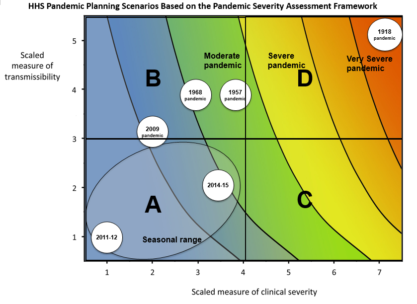
- Does the outbreak have the potential to cause a very severe pandemic?
We can assess the pandemic potential of an epidemic with two critical measurements: the transmissibility and the clinical severity (Fraser et al., 2009, CDC, 2024).
One epidemiological approach to estimating the clinical severity is quantifying the Case Fatality Risk (CFR). CFR is the conditional probability of death given confirmed diagnosis, calculated as the ratio of the cumulative number of deaths from an infectious disease to the number of confirmed diagnosed cases. However, calculating this directly during the course of an epidemic tends to result in a naive or biased CFR given the time delay from onset to death, varying substantially as the epidemic progresses and stabilising at the later stages of the outbreak (Ghani et al., 2005).
More generally, estimating severity can be helpful even outside of a pandemic planning scenario and in the context of routine public health. Knowing whether an outbreak has or had a different severity from the historical record can motivate causal investigations, which could be intrinsic to the infectious agent (e.g., a new, more severe strain) or due to underlying factors in the population (e.g. reduced immunity or morbidity factors) (Lipsitch et al., 2015).
In this tutorial we are going to learn how to use the cfr package to calculate and adjust a CFR estimation using delay distributions from epiparameter or elsewhere, based on the methods developed by Nishiura et al., 2009. We will also explore how we can reuse cfr functions for more severity measurements.
We’ll use the pipe %>% operator from the
magrittr package to connect functions from
cfr, including others from the package
dplyr. Hence, we will load the tidyverse
package which contains both magrittr and
dplyr.
R
# load packages
library(cfr)
library(epiparameter)
library(tidyverse)
library(outbreaks)
The double-colon
The double-colon :: in R lets you call a specific
function from a package without loading the entire package into the
current environment.
For example, dplyr::filter(data, condition) uses the
filter() function from the dplyr
package.
This helps us remember package functions and avoid namespace conflicts.
Have you been a member of an epidemic response team? If yes:
- How did you assess the clinical severity of the outbreak?
- What were the primary sources of bias?
- What did you do to take into account the identified bias?
- What complementary analysis would you do to solve the bias?
Data sources for clinical severity
What data sources can we use to estimate the clinical severity of a disease outbreak? Verity et al., 2020 summarises the spectrum of COVID-19 cases:
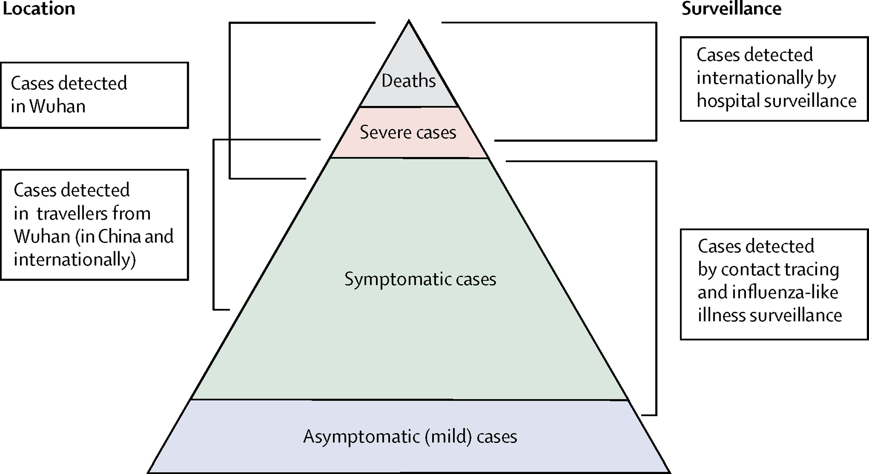
- At the top of the pyramid, those who met the WHO case criteria for severe or critical cases would likely have been identified in the hospital setting, presenting with atypical viral pneumonia. These cases would have been identified in mainland China and among those categorised internationally as local transmission.
- Many more cases are likely to be symptomatic (i.e., with fever, cough, or myalgia) but might not require hospitalisation. These cases would have been identified through links to international travel to high-risk areas and through contact-tracing of contacts of confirmed cases. They might be identifiable through population surveillance of, for example, influenza-like illness.
- The bottom part of the pyramid represents mild (and possibly asymptomatic) cases. These cases might be identifiable through contact tracing and subsequently via serological testing.
Naive CFR
We measure disease severity in terms of case fatality risk (CFR). The CFR is interpreted as the conditional probability of death given confirmed diagnosis, calculated as the ratio of the cumulative number of deaths \(D_{t}\) to the cumulative number of confirmed cases \(C_{t}\) at a certain time \(t\). We can refer it to the naive CFR (also crude or biased CFR, \(b_{t}\)):
\[ naive \, CFR = b_{t} = \frac{D_{t}}{C_{t}} \]
This calculation is naive because it tends to yield a biased and mostly underestimated CFR due to the time-delay from onset to death, only stabilising at the later stages of the outbreak.
To calculate the naive CFR, the cfr package requires an input data frame with three columns named:
datecasesdeaths
Let’s explore the ebola1976 dataset, included in {cfr},
which comes from the first Ebola outbreak in Zaire (now the Democratic
Republic of the Congo) in 1976, as analysed by Camacho et
al. (2014).
R
# Load the Ebola 1976 data provided with the {cfr} package
data("ebola1976")
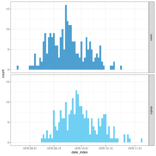
# Plot the incidence of cases and death reports
ebola1976 %>%
incidence2::incidence(
date_index = "date",
counts = c("cases", "deaths")
) %>%
plot()
We’ll frame this episode under the context of an ongoing outbreak with only the first 30 days of data observed (chosen here for illustration, not a required step).
R
# Assume we only have the first 30 days of this data
ebola_30days <- ebola1976 %>%
  dplyr::slice_head(n = 30) %>%
  dplyr::as_tibble()

ebola_30days
OUTPUT
# A tibble: 30 × 3
   date       cases deaths
   <date>     <int>  <int>
 1 1976-08-25     1      0
 2 1976-08-26     0      0
 3 1976-08-27     0      0
 4 1976-08-28     0      0
 5 1976-08-29     0      0
 6 1976-08-30     0      0
 7 1976-08-31     0      0
 8 1976-09-01     1      0
 9 1976-09-02     1      0
10 1976-09-03     1      0
# ℹ 20 more rows
In a real-time analysis, always use the latest data available at the moment.
We need aggregated incidence data
cfr reads aggregated incidence data.
This input data should be aggregated by day, which means one observation per day, containing the daily number of reported cases and deaths. Observations with zero or missing values should also be included, as with all time-series data.
Also, cfr currently works for daily data only, but not for other temporal units of data aggregation, e.g., weeks.
When aggregating cases by day with incidence2, you can
adapt the data for cfr using
cfr::prepare_data() on <incidence2>
objects. For details and an example, consult the cfr
reference manual on preparing
common epidemiological data formats for CFR estimation.
When we apply cfr_static() to data
directly, we are calculating the naive CFR:
R
# Calculate the naive CFR for the first 30 days
cfr::cfr_static(data = ebola_30days)
OUTPUT
  severity_estimate severity_low severity_high
1         0.4740741    0.3875497     0.5617606
The naive CFR estimates the overall disease severity, given the latest data available at the moment, as 0.4740741 with a 95% confidence interval between 0.3875497 and 0.5617606.
Challenge
Download the file sarscov2_cases_deaths.csv and read it into R.
Estimate the naive CFR.
Inspect the format of the data input.
- Does it contain daily data?
- Do the column names match those required by
cfr_static()? - How would you rename the columns in a data frame?
We read the data input using readr::read_csv(). This
function recognises that the column date is a
<date> class vector.
R
# read data
# e.g.: if path to file is data/raw-data/ebola_cases.csv then:
sarscov2_input <-
  readr::read_csv(here::here("data", "raw-data", "sarscov2_cases_deaths.csv"))
R
# Inspect data
sarscov2_input
OUTPUT
# A tibble: 93 × 3
   date       cases_jpn deaths_jpn
   <date>         <dbl>      <dbl>
 1 2020-01-20         1          0
 2 2020-01-21         1          0
 3 2020-01-22         0          0
 4 2020-01-23         1          0
 5 2020-01-24         1          0
 6 2020-01-25         3          0
 7 2020-01-26         3          0
 8 2020-01-27         4          0
 9 2020-01-28         6          0
10 2020-01-29         7          0
# ℹ 83 more rows
We can use dplyr::rename() to adapt the external data to
fit the data input for cfr::cfr_static().
R
# Rename columns before estimating the naive CFR
sarscov2_input %>%
  dplyr::rename(
    cases = cases_jpn,
    deaths = deaths_jpn
  ) %>%
  cfr::cfr_static()
OUTPUT
  severity_estimate severity_low severity_high
1        0.01895208   0.01828832    0.01963342
The naive CFR estimates the overall disease severity, given the latest data available at the moment, as 0.0189521 with a 95% confidence interval between 0.0182883 and 0.0196334.
Biases that affect CFR estimation
Two biases that affect CFR estimation
Lipsitch et al., 2015 describe two potential biases that can affect the estimation of CFR (and their potential solutions):
For diseases with a spectrum of clinical presentations, those cases that come to the attention of public health authorities and are registered into surveillance databases will typically be people with the most severe symptoms who seek medical care, are admitted to a hospital, or die.
Therefore, the CFR will typically be higher among detected cases than among the entire population of cases, given that the latter may include individuals with mild, subclinical, and (under some definitions of “case”) asymptomatic presentations.
During an ongoing epidemic, there is a delay between the time someone dies and the time their death is reported. Therefore, at any given moment in time, the list of cases includes people who will die and whose death has not yet occurred or has occurred but not yet been reported. Thus, dividing the cumulative number of reported deaths by the cumulative number of reported cases at a specific time point during an outbreak will underestimate the true CFR.
The key determinants of the magnitude of the bias are the epidemic growth rate and the distribution of delays from case-reporting to death-reporting; the longer the delays and the faster the growth rate, the greater the bias.
In this tutorial episode, we are going to focus on solutions to deal with this specific bias using cfr!
Improving an early epidemiological assessment of a delay-adjusted CFR is crucial for determining virulence, shaping the level and choices of public health intervention, and providing advice to the general public.
In 2009, during the swine-flu outbreak caused by Influenza A (H1N1), Mexico had an early biased estimation of the CFR. Initial reports from the government of Mexico suggested a virulent infection, whereas, in other countries, the same virus was perceived as mild (TIME, 2009).
In the USA and Canada, no deaths were attributed to the virus in the first ten days following the World Health Organization’s declaration of a public health emergency. Even under similar circumstances at the early stage of the global pandemic, public health officials, policymakers and the general public want to know the virulence of an emerging infectious agent.
Garske et al., 2009 assess the challenges to estimate the severity of this pandemic, emphasising that accurately capturing the cases for the denominator can improve the capacity to obtain informative CFR estimates.
Delay-adjusted CFR
Nishiura et al., 2009 developed a method that considers the time delay from the onset of symptoms to death.
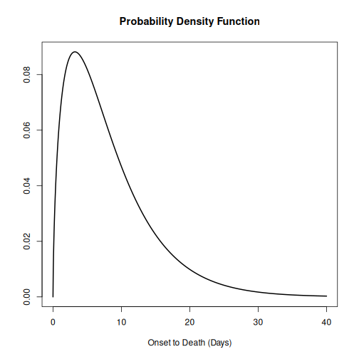
Real-time outbreaks may have a number of deaths that are insufficient to determine the time distribution between onset and death. Therefore, we can estimate the distribution delay from historical outbreaks or reuse the ones accessible via R packages like epiparameter or epireview, which collect them from published scientific literature. For a step-by-step guide, read the tutorial episode on how to access epidemiological delays.
Let’s use epiparameter:
R
# Get delay distribution
onset_to_death_ebola <- epiparameter::epiparameter_db(
  disease = "Ebola",
  epi_name = "onset_to_death",
  single_epiparameter = TRUE
)

# Plot <epiparameter> object
plot(onset_to_death_ebola, xlim = c(0, 40))
To calculate the delay-adjusted CFR, we can use the
cfr_static() function with the data and
delay_density arguments.
R
# Calculate the delay-adjusted CFR
# for the first 30 days
cfr::cfr_static(
  data = ebola_30days,
  delay_density = function(x) density(onset_to_death_ebola, x)
)
OUTPUT
  severity_estimate severity_low severity_high
1            0.9502        0.881        0.9861
The delay-adjusted CFR estimates the overall disease severity, given the latest data available at the moment, as 0.9502 with a 95% confidence interval between 0.881 and 0.9861, substantially higher than the naive estimate. This larger value reflects the correction for deaths that are still to be reported among the cases observed in the first 30 days.
How does {cfr} work?
If you want to gain familiarity and learn how delays are accounted for when estimating CFR, you can read the episode on How to adjust the CFR for delays in the “More Resources” section of this tutorial’s website.
First, read the guide on How to adjust the CFR for delays. Optionally, review the definition of a probability density function (PDF) in the episode on Use delay distributions in analysis.
You will find that the core calculation is to get the total
expected number of cases with known outcomes by time
t. This is to account for the fact that some
fraction of recent cases haven’t had time to resolve to death/recovery
yet. It is expressed by the term:
\[ \sum_{i = 0}^t\sum_{j = 0}^\infty c_i f_{j - i} \]
where:
- \(c_i\) is the number of new confirmed cases on day i
- \(f_s\) the conditional probability density function for the delay of \(s\) days, from onset to death, given death.
It sums the incident cases \(c_i\) over all onset days \(i\) up to \(t\), and for each one, weights it by \(f_{j-i}\), the probability of the outcome becoming known on day \(j\), summed over all days \(j\).
For each day i, cfr computes the
expected number of outcomes arising from that day’s
newly observed incident cases: the outcomes expected “at” day
i. These per-day expected outcomes are then summed
cumulatively across the full history up to time t to obtain
the total expected number of outcomes “by” time
t.
First step: the expected number of outcomes at day i
When using <epiparameter> class objects, the
function density() can be applied to obtain the
corresponding probability density function for incident cases “at” day
i.
For example, at day 0, the expected outcomes are equal to:
- \(c_0 \times (f_0)\): the number of incident cases on day 0 times the density at day 0.
R
# By Day 0, the expected outcomes are:
ebola_30days$cases[1] *
  density(onset_to_death_ebola, at = 0)
OUTPUT
[1] 0Notice that ebola_30days$cases[1] represent the number
of incident cases on day 0 to fit the notation from the
equation above.
At day 1, the expected outcomes are equal to:
- \(c_0 \times (f_1)\): the number of incident cases on day 0 times the density at day 1, plus
- \(c_1 \times (f_0)\): the number of incident cases on day 1 times the density at day 0.
R
# By Day 1, the expected outcomes are:
ebola_30days$cases[1] *
  density(onset_to_death_ebola, at = 1) +
  ebola_30days$cases[2] *
    density(onset_to_death_ebola, at = 0)
OUTPUT
[1] 0.06495664At day 2, the expected outcomes are equal to:
- \(c_0 \times (f_2)\): the number of incident cases on day 0 times the density at day 2, plus
- \(c_1 \times (f_1)\): the number of incident cases on day 1 times the density at day 1, plus
- \(c_2 \times (f_0)\): the number of incident cases on day 2 times the density at day 0.
R
# By Day 3, the expected outcomes are:
ebola_30days$cases[1] *
  density(onset_to_death_ebola, at = 2) +
  ebola_30days$cases[2] *
    density(onset_to_death_ebola, at = 1) +
  ebola_30days$cases[3] *
    density(onset_to_death_ebola, at = 0)
OUTPUT
[1] 0.08295091Notice that the delay index shifts by one day at a time: the most recent cases (day \(t\)) are weighted by \(f_0\), the previous day’s cases by \(f_1\), and so on, with each earlier day moving one step further along the delay distribution.
Since the input value in at varies by day for incident
cases of a given day (at = 0, at = 1,
at = 2, …), the density() needs to be
expressed as a function of x. cfr will then
draw values accordingly, as shown below:
R
# {cfr} uses the density of the distribution at different values of x
function(x) density(onset_to_death_ebola, at = x)
Internally, for the first 3 days (day 0, day 1, and day 2), the
function cfr::estimate_outcomes() performs this
calculation:
R
cfr::estimate_outcomes(
  data = ebola_30days,
  delay_density = function(x) density(onset_to_death_ebola, at = x)
) %>%
  slice_head(n = 3) %>%
  pull(estimated_outcomes)
OUTPUT
[1] 0.00000000 0.06495664 0.08295091The values printed above are estimate_outcomes for the
corresponding day.
Second step: the total expected number of outcomes “by” time t
These per-day expected outcomes are then summed cumulatively across
the full history up to time t to obtain the total
expected number of outcomes “by” time t.
By day 2, the total expected outcomes are equal to:
- \(c_0 \times (f_0 + f_1 + f_2)\): expected outcomes from day 0’s incident cases, by day 2
- \(c_1 \times (f_0 + f_1)\): expected outcomes from day 1’s incident cases, by day 2
- \(c_2 \times (f_0)\): expected outcomes from day 2’s incident cases, by day 2
Summing these terms gives the total expected outcomes by day 2. This
match the double summation shown above. This total is used to calculate
the underestimation factor (u_t), the
fraction of cases whose outcomes are already known.
Use the epiparameter class
When using an <epiparameter> class object we can
use this expression as a template:
function(x) density(<EPIPARAMETER_OBJECT>, x)
For distribution functions with parameters not available in epiparameter, we suggest two alternatives:
Create an
<epiparameter>class object, to plug into other R packages of the outbreak analytics pipeline. Read the reference documentation ofepiparameter::epiparameter()Read cfr vignette for a primer on working with delay distributions.
For cfr_static() and all functions in the
cfr_*() family, the most appropriate distributions to use
are discrete ones. This is because cfr
operates on count data in discrete time: daily case and death
counts.
We can assume that evaluating the Probability Density Function (PDF) of a continuous distribution is equivalent to the Probability Mass Function (PMF) of the equivalent discrete distribution.
However, this assumption may not be appropriate for distributions
with larger peaks. For instance, diseases with an onset-to-death
distribution that is strongly peaked with a low variance. In such cases,
the average disparity between the PDF and PMF is expected to be more
pronounced compared to distributions with broader spreads. One way to
deal with this is to discretise the continuous distribution using
epiparameter::discretise() to an
<epiparameter> object.
R
onset_to_death_ebola %>%
  epiparameter::discretise() %>%
  plot(xlim = c(0, 40))

Challenge
Use the same file from the previous challenge (sarscov2_cases_deaths.csv).
Estimate the delay-adjusted CFR using the appropriate distribution delay. Then:
- Compare the naive and the delay-adjusted CFR solutions!
- Find the appropriate
<epiparameter>object!
We use epiparameter to access a delay distribution for the SARS-CoV-2 aggregated incidence data:
R
library(epiparameter)

sarscov2_delay <-
  epiparameter::epiparameter_db(
    disease = "covid",
    epi_name = "onset to death",
    single_epiparameter = TRUE
  )
We read the data input using readr::read_csv(). This
function recognises that the column date is a
<date> class vector.
R
# read data
# e.g.: if path to file is data/raw-data/ebola_cases.csv then:
sarscov2_input <-
  readr::read_csv(here::here("data", "raw-data", "sarscov2_cases_deaths.csv"))
R
# Inspect data
sarscov2_input
OUTPUT
# A tibble: 93 × 3
   date       cases_jpn deaths_jpn
   <date>         <dbl>      <dbl>
 1 2020-01-20         1          0
 2 2020-01-21         1          0
 3 2020-01-22         0          0
 4 2020-01-23         1          0
 5 2020-01-24         1          0
 6 2020-01-25         3          0
 7 2020-01-26         3          0
 8 2020-01-27         4          0
 9 2020-01-28         6          0
10 2020-01-29         7          0
# ℹ 83 more rows
We can use the dplyr::rename() to adapt the external
data to fit the data input for cfr_static().
R
# Rename columns before estimating the delay-adjusted CFR
sarscov2_input %>%
  dplyr::rename(
    cases = cases_jpn,
    deaths = deaths_jpn
  ) %>%
  cfr::cfr_static(
    delay_density = function(x) density(sarscov2_delay, x)
  )
OUTPUT
  severity_estimate severity_low severity_high
1            0.0734        0.071        0.0759
Task: Interpret the comparison between the naive and delay-adjusted CFR estimates.
An early-stage CFR estimate
The naive estimate is useful to get an overall severity estimate of the outbreak (so far). Once the outbreak has ended or has progressed such that more deaths are reported, the estimated CFR is then closest to the ‘true’ unbiased CFR.
On the other hand, the delay-adjusted estimate can assess the severity of an emerging infectious disease earlier in an outbreak given a more reliable assessment of the severity than the naive CFR.
We can explore the early determination of the
delay-adjusted CFR using the cfr_rolling()
function.
cfr_rolling() is a utility function that automatically
calculates CFR for each day of the outbreak with the data available up
to that day, saving the user time.
cfr_rolling() shows the estimated CFR on each outbreak
day, given that future data on cases and deaths is unavailable at the
time. The final value of cfr_rolling() estimates is
identical to cfr_static() on the same data.
R
# for all the 73 days in the Ebola dataset
# Calculate the rolling daily naive CFR
rolling_cfr_naive <- cfr::cfr_rolling(data = ebola1976)
OUTPUT
`cfr_rolling()` is a convenience function to help understand how additional data influences the overall (static) severity. Use `cfr_time_varying()` instead to estimate severity changes over the course of the outbreak.R
# for all the 73 days in the Ebola dataset
# Calculate the rolling daily delay-adjusted CFR
rolling_cfr_adjusted <- cfr::cfr_rolling(
  data = ebola1976,
  delay_density = function(x) density(onset_to_death_ebola, x)
)
OUTPUT
`cfr_rolling()` is a convenience function to help understand how additional data influences the overall (static) severity. Use `cfr_time_varying()` instead to estimate severity changes over the course of the outbreak.OUTPUT
Some daily ratios of total deaths to total cases with known outcome are below 0.01%: some CFR estimates may be unreliable.FALSEWith utils::tail(), we view the latest CFR estimates.
The naive and delay-adjusted estimates have overlapping ranges of 95%
confidence intervals.
R
# Print the tail of the data frame
utils::tail(rolling_cfr_naive)
utils::tail(rolling_cfr_adjusted)
Now, let’s visualise both results in a time series. How would the naive and delay-adjusted CFR estimates perform in real time?
R
# bind by rows both output data frames
dplyr::bind_rows(
  list(
    naive = rolling_cfr_naive,
    adjusted = rolling_cfr_adjusted
  ),
  .id = "method"
) %>%
  # visualise both adjusted and unadjusted rolling estimates
  ggplot() +
  geom_ribbon(
    aes(
      date,
      ymin = severity_low,
      ymax = severity_high,
      fill = method
    ),
    alpha = 0.2, show.legend = FALSE
  ) +
  geom_line(
    aes(date, severity_estimate, colour = method)
  )
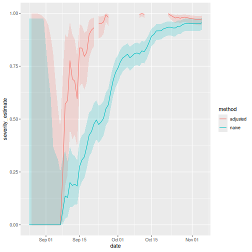
The red and blue lines represent the delay-adjusted and naive CFR, respectively, throughout the outbreak. The bands around them represent the 95% confidence intervals (95% CI).
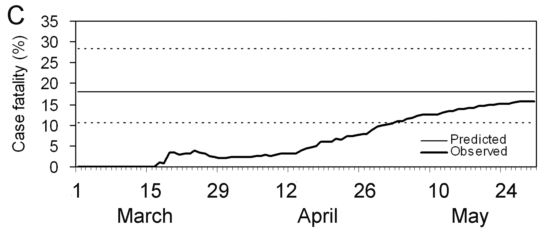
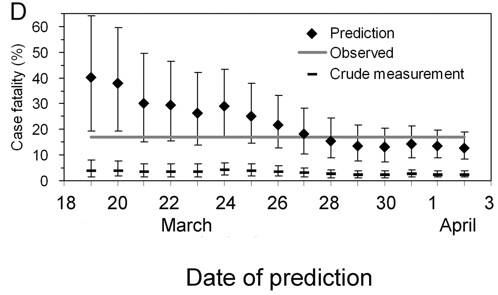
Notice that this delay-adjusted calculation is particularly useful when an epidemic curve of confirmed cases is the only data available (i.e. when individual data from onset to death are unavailable, especially during the early stage of the epidemic). When there are few deaths or none at all, an assumption has to be made for the delay distribution from onset to death, e.g. from literature based on previous outbreaks. Nishiura et al., 2009 depict this in the figures with data from the SARS outbreak in Hong Kong, 2003.
Figures A and B show the cumulative numbers of cases and deaths of SARS, and Figure C shows the observed (biased) CFR estimates as a function of time, i.e. the cumulative number of deaths over cases at time \(t\). Due to the delay from the onset of symptoms to death, the biased estimate of CFR at time \(t\) underestimates the realised CFR at the end of an outbreak (i.e. 302/1755 = 17.2 %).
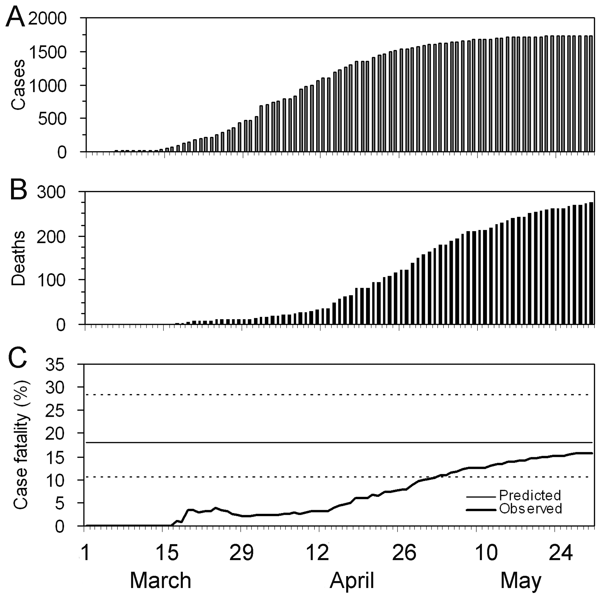
Nevertheless, even by only using the observed data for the period
March 19 to April 2, cfr_static() can yield an appropriate
prediction (Figure D), e.g. the delay-adjusted CFR at March 27 is 18.1 %
(95% CI: 10.5, 28.1). An overestimation is seen in the very early stages
of the epidemic, but the 95% confidence limits in the later stages
include the realised CFR (i.e. 17.2 %).
Interpret the early-stage CFR estimate
Based on the figure above of the naive and adjusted rolling CFR:
- How many days apart are the dates on which the 95% CI of the delay-adjusted CFR and the 95% CI of the naive CFR each first cross the CFR estimated at the end of the outbreak?
Discuss:
- What are the Public health policy implications of having a delay-adjusted CFR estimate?
We can either use a visual inspection or analyse the output data frames.
The CFR estimated at the end of the outbreak is:
R
utils::tail(rolling_cfr_naive, n = 1)
OUTPUT
         date severity_estimate severity_low severity_high
73 1976-11-05 0.955102 0.9210866 0.9773771Checklist
With cfr, we estimate the CFR as the proportion of deaths among confirmed cases.
By only using confirmed cases, it is clear that all cases that do not seek medical treatment or are not notified will be missed, as well as all asymptomatic cases. This means that the CFR estimate is higher than the proportion of deaths among the infected.
cfr method aims to obtain an unbiased estimator “well before” observing the entire course of the outbreak. For this, cfr uses the underestimation factor \(u_{t}\) to estimate the unbiased CFR \(p_{t}\) using maximum-likelihood methods, given the sampling process defined by Nishiura et al., 2009.
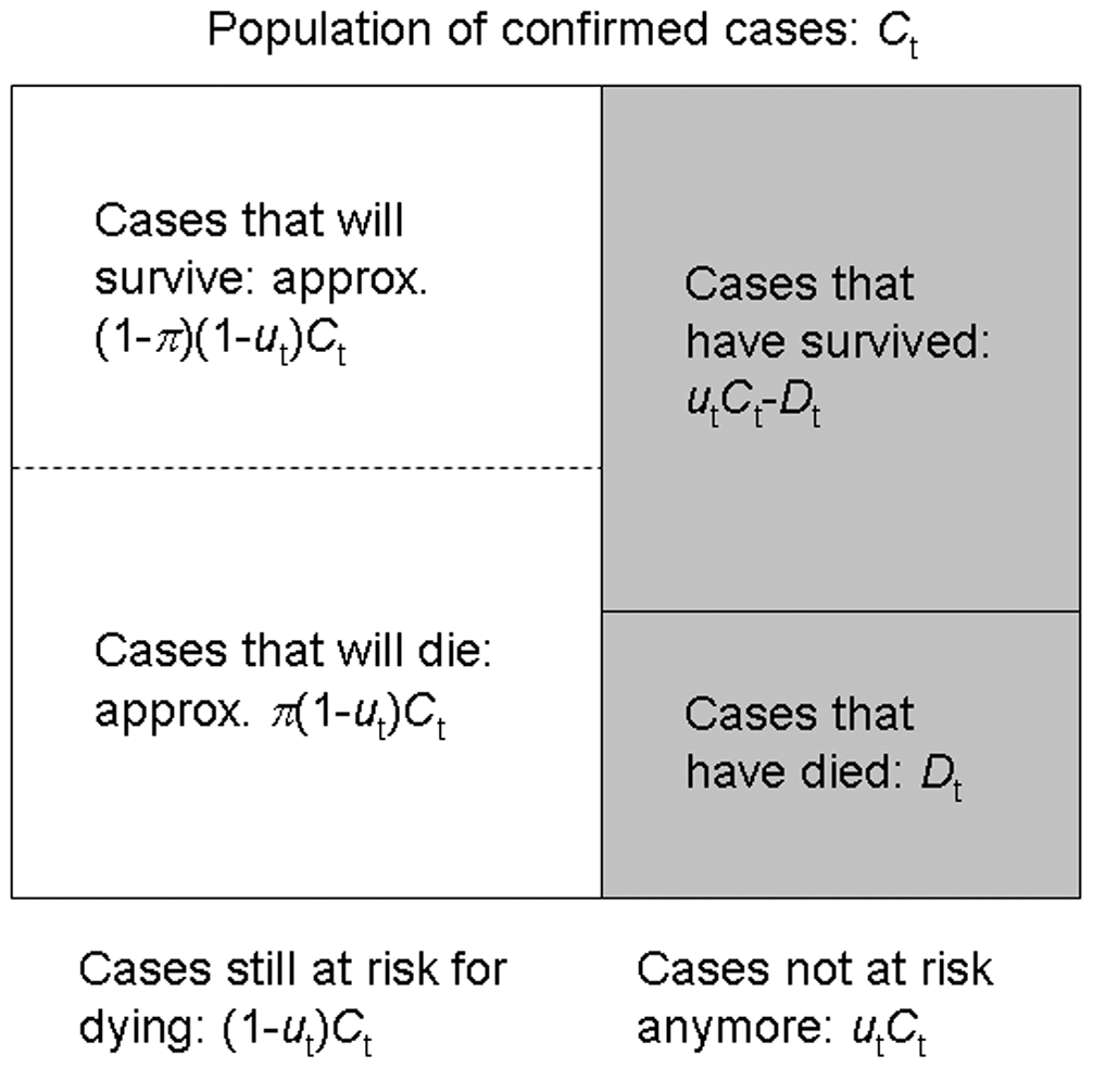
From aggregated incidence data, at time \(t\) we know the cumulative number of confirmed cases and deaths, \(C_{t}\) and \(D_{t}\), and wish to estimate the unbiased CFR \(\pi\), by way of the factor of underestimation \(u_{t}\).
If we knew the factor of underestimation \(u_{t}\) we could specify the size of the population of confirmed cases no longer at risk (\(u_{t}C_{t}\), shaded), although we do not know which surviving individuals belong to this group. A proportion \(\pi\) of those in the group of cases still at risk (size \((1- u_{t})C_{t}\), unshaded) is expected to die.
Because each case no longer at risk had an independent probability of dying, \(\pi\), the number of deaths, \(D_{t}\), is a sample from a binomial distribution with sample size \(u_{t}C_{t}\), and probability of dying \(p_{t}\) = \(\pi\).
This is represented by the following likelihood function to obtain the maximum likelihood estimate of the unbiased CFR \(p_{t}\) = \(\pi\):
\[ {\sf L}(\pi | C_{t},D_{t},u_{t}) = \log{\dbinom{u_{t}C_{t}}{D_{t}}} + D_{t} \log{\pi} + (u_{t}C_{t} - D_{t})\log{(1 - \pi)}, \]
This estimation is performed by the internal function
?cfr:::estimate_severity().
- The delay-adjusted CFR does not address all sources of error in data like the underdiagnosis of infected individuals.
Challenges
Aggregated data differ from linelists
Aggregated incidence data differs from linelist data, where each observation contains individual-level data.
R
outbreaks::ebola_sierraleone_2014 %>% as_tibble()
OUTPUT
# A tibble: 11,903 × 8
      id   age sex   status    date_of_onset date_of_sample district chiefdom
   <int> <dbl> <fct> <fct>     <date>        <date>         <fct>    <fct>
 1     1    20 F     confirmed 2014-05-18    2014-05-23     Kailahun Kissi Teng
 2     2    42 F     confirmed 2014-05-20    2014-05-25     Kailahun Kissi Teng
 3     3    45 F     confirmed 2014-05-20    2014-05-25     Kailahun Kissi Tonge
 4     4    15 F     confirmed 2014-05-21    2014-05-26     Kailahun Kissi Teng
 5     5    19 F     confirmed 2014-05-21    2014-05-26     Kailahun Kissi Teng
 6     6    55 F     confirmed 2014-05-21    2014-05-26     Kailahun Kissi Teng
 7     7    50 F     confirmed 2014-05-21    2014-05-26     Kailahun Kissi Teng
 8     8     8 F     confirmed 2014-05-22    2014-05-27     Kailahun Kissi Teng
 9     9    54 F     confirmed 2014-05-22    2014-05-27     Kailahun Kissi Teng
10    10    57 F     confirmed 2014-05-22    2014-05-27     Kailahun Kissi Teng
# ℹ 11,893 more rowsHow to rearrange my input data?
Rearranging the input data for data analysis can take most of the time. To get ready-to-analyse aggregated incidence data, we encourage you to use incidence2!
First, in the Get
started vignette from the incidence2 package, explore
how to use the date_index argument when reading a linelist
with dates in multiple column.
Then, refer to the cfr reference manual on Prepare
common epidemiological data formats for CFR estimation on how to use
the cfr::prepare_data() function from incidence2
objects.
R
# Load packages
library(cfr)
library(epiparameter)
library(incidence2)
library(outbreaks)
library(tidyverse)

# Access delay distribution
mers_delay <- epiparameter::epiparameter_db(
  disease = "mers",
  epi_name = "onset to death",
  single_epiparameter = TRUE
)

# Read linelist
mers_korea_2015$linelist %>%
  as_tibble() %>%
  select(starts_with("dt_"))
OUTPUT
# A tibble: 162 × 6
   dt_onset   dt_report  dt_start_exp dt_end_exp dt_diag    dt_death
   <date>     <date>     <date>       <date>     <date>     <date>
 1 2015-05-11 2015-05-19 2015-04-18   2015-05-04 2015-05-20 NA
 2 2015-05-18 2015-05-20 2015-05-15   2015-05-20 2015-05-20 NA
 3 2015-05-20 2015-05-20 2015-05-16   2015-05-16 2015-05-21 2015-06-04
 4 2015-05-25 2015-05-26 2015-05-16   2015-05-20 2015-05-26 NA
 5 2015-05-25 2015-05-27 2015-05-17   2015-05-17 2015-05-26 NA
 6 2015-05-24 2015-05-28 2015-05-15   2015-05-17 2015-05-28 2015-06-01
 7 2015-05-21 2015-05-28 2015-05-16   2015-05-17 2015-05-28 NA
 8 2015-05-26 2015-05-29 2015-05-15   2015-05-15 2015-05-29 NA
 9 NA         2015-05-29 2015-05-15   2015-05-17 2015-05-29 NA
10 2015-05-21 2015-05-29 2015-05-16   2015-05-16 2015-05-29 NA
# ℹ 152 more rows
R
# Use {incidence2} to count daily incidence
mers_incidence <- mers_korea_2015$linelist %>%
  # convert to incidence2 object
  incidence(date_index = c("dt_onset", "dt_death")) %>%
  # complete dates from first to last
  incidence2::complete_dates()

# Inspect incidence2 output
mers_incidence
OUTPUT
# incidence:  72 x 3
# count vars: dt_death, dt_onset
   date_index count_variable count
   <date>     <chr>          <int>
 1 2015-05-11 dt_death           0
 2 2015-05-11 dt_onset           1
 3 2015-05-12 dt_death           0
 4 2015-05-12 dt_onset           0
 5 2015-05-13 dt_death           0
 6 2015-05-13 dt_onset           0
 7 2015-05-14 dt_death           0
 8 2015-05-14 dt_onset           0
 9 2015-05-15 dt_death           0
10 2015-05-15 dt_onset           0
# ℹ 62 more rows
R
# Prepare data from {incidence2} to {cfr}
mers_incidence %>%
  cfr::prepare_data(
    cases_variable = "dt_onset",
    deaths_variable = "dt_death"
  )
OUTPUT
         date deaths cases
1  2015-05-11      0     1
2  2015-05-12      0     0
3  2015-05-13      0     0
4  2015-05-14      0     0
5  2015-05-15      0     0
6  2015-05-16      0     0
7  2015-05-17      0     1
8  2015-05-18      0     1
9  2015-05-19      0     0
10 2015-05-20      0     5
11 2015-05-21      0     6
12 2015-05-22      0     2
13 2015-05-23      0     4
14 2015-05-24      0     2
15 2015-05-25      0     3
16 2015-05-26      0     1
17 2015-05-27      0     2
18 2015-05-28      0     1
19 2015-05-29      0     3
20 2015-05-30      0     5
21 2015-05-31      0    10
22 2015-06-01      2    16
23 2015-06-02      0    11
24 2015-06-03      1     7
25 2015-06-04      1    12
26 2015-06-05      1     9
27 2015-06-06      0     7
28 2015-06-07      0     7
29 2015-06-08      2     6
30 2015-06-09      0     1
31 2015-06-10      2     6
32 2015-06-11      1     3
33 2015-06-12      0     0
34 2015-06-13      0     2
35 2015-06-14      0     0
36 2015-06-15      0     1
R
# Estimate delay-adjusted CFR
mers_incidence %>%
  cfr::prepare_data(
    cases_variable = "dt_onset",
    deaths_variable = "dt_death"
  ) %>%
  cfr::cfr_static(delay_density = function(x) density(mers_delay, x))
OUTPUT
  severity_estimate severity_low severity_high
1 0.1377 0.0716 0.2288Severity heterogeneity
The CFR may differ across populations (e.g. age, space, treatment); quantifying these heterogeneities can help target resources appropriately and compare different care regimens (Cori et al., 2017).
Use the cfr::covid_data data frame to estimate a
delay-adjusted CFR stratified by country.
One way to do a stratified analysis is to apply a model to
nested data. This {tidyr}
vignette shows you how to apply the group_by() +
nest() to nest data, and then mutate() +
map() to apply the model.
R
library(cfr)
library(epiparameter)
library(tidyverse)

covid_data %>% glimpse()
OUTPUT
Rows: 20,786
Columns: 4
$ date    <date> 2020-01-03, 2020-01-03, 2020-01-03, 2020-01-03, 2020-01-03, 2…
$ country <chr> "Argentina", "Brazil", "Colombia", "France", "Germany", "India…
$ cases   <dbl> 0, 0, 0, 0, 0, 0, 0, 0, 0, 0, 0, 0, 0, 0, 0, 0, 0, 0, 0, 0, 0,…
$ deaths  <dbl> 0, 0, 0, 0, 0, 0, 0, 0, 0, 0, 0, 0, 0, 0, 0, 0, 0, 0, 0, 0, 0,…
R
delay_onset_death <-
  epiparameter::epiparameter_db(
    disease = "covid",
    epi_name = "onset to death",
    single_epiparameter = TRUE
  )

covid_data %>%
  group_by(country) %>%
  nest() %>%
  mutate(
    temp =
      map(
        .x = data,
        .f = cfr::cfr_static,
        delay_density = function(x) density(delay_onset_death, x)
      )
  ) %>%
  unnest(cols = temp)
OUTPUT
# A tibble: 19 × 5
# Groups:   country [19]
   country        data     severity_estimate severity_low severity_high
   <chr>          <list>               <dbl>        <dbl>         <dbl>
 1 Argentina      <tibble>            0.0133       0.0133        0.0133
 2 Brazil         <tibble>            0.0195       0.0195        0.0195
 3 Colombia       <tibble>            0.0225       0.0224        0.0226
 4 France         <tibble>            0.0044       0.0044        0.0044
 5 Germany        <tibble>            0.0045       0.0045        0.0045
 6 India          <tibble>            0.0119       0.0119        0.0119
 7 Indonesia      <tibble>            0.024        0.0239        0.0241
 8 Iran           <tibble>            0.0191       0.0191        0.0192
 9 Italy          <tibble>            0.0075       0.0075        0.0075
10 Mexico         <tibble>            0.0461       0.046         0.0462
11 Peru           <tibble>            0.0502       0.0501        0.0504
12 Poland         <tibble>            0.0186       0.0186        0.0187
13 Russia         <tibble>            0.0182       0.0182        0.0182
14 South Africa   <tibble>            0.0254       0.0253        0.0255
15 Spain          <tibble>            0.0087       0.0087        0.0087
16 Turkey         <tibble>            0.006        0.006         0.006
17 Ukraine        <tibble>            0.0204       0.0203        0.0205
18 United Kingdom <tibble>            0.009        0.009         0.009
19 United States  <tibble>            0.0111       0.0111        0.0111
Great! Now you can use similar code for any other stratified analysis like age, regions or more!
But, how can we interpret that there is a country variability of severity from the same diagnosed pathogen?
Local factors like testing capacity, the case definition, and sampling regime can affect the report of cases and deaths, thus affecting case ascertainment. Take a look to the cfr vignette on Estimating the proportion of cases that are ascertained during an outbreak!
Appendix
The cfr package has a function called
cfr_time_varying() with functionality that differs from
cfr_rolling().
When to use cfr_rolling()?
cfr_rolling() shows the estimated CFR on each outbreak
day, given that future data on cases and deaths is unavailable at the
time. The final value of cfr_rolling() estimates is
identical to cfr_static() on the same data.
Remember, as shown above, cfr_rolling() is helpful to
get early-stage CFR estimates and check whether an outbreak’s CFR
estimate has stabilised. Thus, cfr_rolling() is not
sensitive to the length or size of the epidemic.
When to use
cfr_time_varying()?
On the other hand, cfr_time_varying() calculates the CFR
over a moving window and helps to understand changes in CFR due to
changes in the epidemic, e.g. due to a new variant or increased immunity
from vaccination.
However, cfr_time_varying() is sensitive to sampling
uncertainty. Thus, it is sensitive to the size of the outbreak. The
higher the number of cases with expected outcomes on a given day, the
more reasonable estimates of the time-varying CFR we will get.
For example, with 100 cases, the fatality risk estimate will, roughly
speaking, have a 95% confidence interval ±10% of the mean estimate
(binomial CI). So if we have >100 cases with expected outcomes on
a given day, we can get reasonable estimates of the time varying
CFR. But if we only have >100 cases over the course of the whole
epidemic, we probably need to rely on cfr_rolling()
that uses the cumulative data.
We invite you to read this vignette
about the cfr_time_varying() function.
More severity measures
Suppose we need to assess the clinical severity of the epidemic in a context different from surveillance data, like the severity among cases that arrive at hospitals or cases you collected from a representative serological survey.
Using cfr, we can change the inputs for the numerator
(cases) and denominator (deaths) to estimate
more severity measures like the Infection fatality risk (IFR) or the
Hospitalisation Fatality Risk (HFR). We can follow this analogy:
If for a Case fatality risk (CFR), we require:
- case and death incidence data, with a
- case-to-death delay distribution (or close approximation, such as symptom onset-to-death).
Then, the Infection fatality risk (IFR) requires:
- infection and death incidence data, with an
- exposure-to-death delay distribution (or close approximation).
Similarly, the Hospitalisation Fatality Risk (HFR) requires:
- hospitalisation and death incidence data, and a
- hospitalisation-to-death delay distribution.
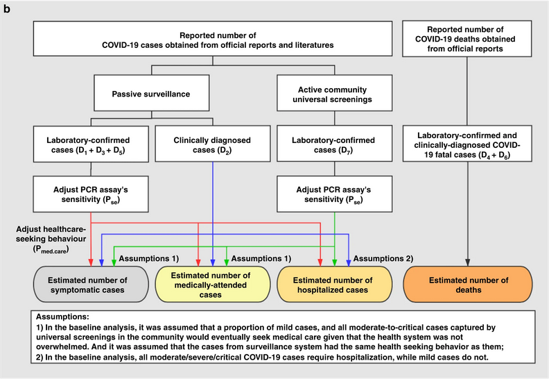
Yang et al., 2020 summarises different definitions and data sources:
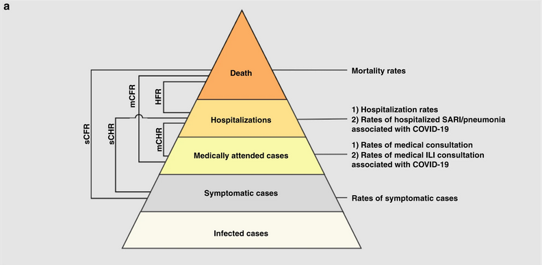
- sCFR symptomatic case-fatality risk,
- sCHR symptomatic case-hospitalisation risk,
- mCFR medically attended case-fatality risk,
- mCHR medically attended case-hospitalisation risk,
- HFR hospitalisation-fatality risk.
Use cfr to estimate severity
Use
cfr_static()to estimate the overall CFR with the latest data available.Use
cfr_rolling()to show what the estimated CFR would be on each day of the outbreak.Use the
delay_densityargument to adjust the CFR by the corresponding delay distribution.