ColOpenData can be used to access open geospatial data from Colombia. This data is retrieved from the National Geostatistical Framework (MGN), published by Departamento Administrativo Nacional de Estadística (DANE). The MGN contains the political-administrative division and is used to reference census statistical information.
This package contains the 2018’s version of the MGN, which also
included a summarized version of the National Population and Dwelling
Census (CNPV) in different aggregation levels. Each level is stored in a
different dataset, which can be retrieved using the
download_geospatial() function, which requires three
arguments:
-
spatial_levelcharacter with the spatial level to be consulted -
simplifiedlogical for indicating if the downloaded spatial data should be a simplified version of the geometries. Simplified versions are lighter but less precise, and are recommended for easier applications like plots. Default is . -
include_geomlogical for including (or not) geometry. Default isTRUE -
include_cnpvlogical for including (or not) CNPV demographic and socioeconomic information Default isTRUE.
Available levels of aggregation come from the official spatial division provided by DANE, with their names corresponding to:
| Code | Level | Name |
|---|---|---|
| DPTO | Department | DANE_MGN_2018_DPTO |
| MPIO | Municipality | DANE_MGN_2018_MPIO |
| MPIOCL | Municipality including Class | DANE_MGN_2018_MPIOCL |
| MZN | Block | DANE_MGN_2018_MZN |
| SECR | Rural Sector | DANE_MGN_2018_SECR |
| SECU | Urban Sector | DANE_MGN_2018_SECU |
| SETR | Rural Section | DANE_MGN_2018_SETR |
| SETU | Urban Section | DANE_MGN_2018_SETU |
| ZU | Urban Zone | DANE_MGN_2018_ZU |
In this vignette you will learn:
- How to download geospatial data using ColOpenData.
- How to use census data included in geospatial datasets.
- How to visualize spatial data using leaflet and ggplot2.
We will be using geospatial data at the level of Department (“dpto”) and we will calculate the percentage of dwellings with internet connection at each department. Later, we will build some plots using the previously mentioned approaches for dynamic and static plots.
We will start by importing the needed libraries.
Disclaimer: all data is loaded to the environment in the user’s R session, but is not downloaded to user’s computer. Spatial datasets can be very long and might take a while to be loaded in the environment
Downloading geospatial data
First, we download the data using the function
download_geospatial(), including the geometries and the
census related information. The simplified parameter is
used to download a lighter version, since simple plots do not require
precise spatial information.
dpto <- download_geospatial(
spatial_level = "dpto",
simplified = TRUE,
include_geom = TRUE,
include_cnpv = TRUE
)
#> This might take a while
#> ColOpenData provides open data derived from Departamento Administrativo
#> Nacional de Estadística (DANE), and Instituto de Hidrología,
#> Meteorología y Estudios Ambientales (IDEAM) but with modifications for
#> specific functional needs. These changes may alter the structure,
#> format, or content, meaning the data does not reflect the official
#> dataset. The package is developed independently, with no endorsement or
#> involvement from these institutions or any Colombian government body.
#> The authors of ColOpenData are not liable for how users utilize the
#> data, and users areresponsible for any outcomes from their use or
#> analysis of the data.
#> Stored by Universidad de Los Andes under the Epiverse TRACE iniative.
head(dpto)
#> Simple feature collection with 6 features and 88 fields
#> Geometry type: MULTIPOLYGON
#> Dimension: XY
#> Bounding box: xmin: -77.92834 ymin: -0.70584 xmax: -66.84722 ymax: 6.324304
#> Geodetic CRS: WGS 84
#> codigo_departamento departamento version area latitud longitud
#> 1 18 Caquetá 2018 90103008160 0.7985562 -73.95947
#> 2 19 Cauca 2018 31242914793 2.3968339 -76.82423
#> 3 86 Putumayo 2018 25976283135 0.4522600 -75.85591
#> 4 76 Valle del Cauca 2018 20665544525 3.8588583 -76.51869
#> 5 94 Guainía 2018 71289354481 2.7278429 -68.81661
#> 6 99 Vichada 2018 100063370591 4.7135571 -69.41400
#> encuestas enc_etnico enc_no_etnico enc_resguardo_indigena enc_comun_negras
#> 1 163381 1117 162264 1117 0
#> 2 622959 83033 539926 70827 12206
#> 3 147797 4704 143093 4659 45
#> 4 1674673 18250 1656423 3618 14632
#> 5 13059 3675 9384 3675 0
#> 6 24915 6870 18045 6870 0
#> enc_area_protegida enc_area_no_protegida un_vivienda un_mixto un_no_res
#> 1 544 162837 132937 5429 24804
#> 2 226 622733 446806 10837 165011
#> 3 1389 146408 107456 3397 36789
#> 4 21431 1653242 1410067 39096 224820
#> 5 532 12527 11111 293 1553
#> 6 171 24744 20051 747 4016
#> un_lea un_mixto_no_res_industria un_mixto_no_res_comercio
#> 1 211 96 3860
#> 2 324 328 6147
#> 3 173 67 2572
#> 4 690 1920 22705
#> 5 102 12 154
#> 6 101 12 548
#> un_mixto_no_res_servicios un_mixto_no_res_agro un_mixto_no_res_sin_info
#> 1 1117 243 113
#> 2 2276 2016 70
#> 3 717 29 12
#> 4 11986 2357 128
#> 5 106 6 15
#> 6 151 22 14
#> un_no_res_industria un_no_res_comercio un_no_res_servicios un_no_res_agro
#> 1 160 5422 2511 3052
#> 2 810 10334 9455 43342
#> 3 188 4402 2485 6665
#> 4 5572 50097 40191 32665
#> 5 15 244 263 24
#> 6 13 601 418 25
#> un_no_res_institucional un_no_res_lote un_no_res_parque un_no_res_minero
#> 1 1250 10099 678 12
#> 2 3515 86486 3155 105
#> 3 1428 18445 368 74
#> 4 5452 67080 6881 169
#> 5 149 597 35 7
#> 6 220 2290 109 3
#> un_no_res_proteccion u_no_res_construccion u_no_res_sin_info viviendas
#> 1 96 1453 71 138366
#> 2 969 6596 244 457643
#> 3 319 2334 81 110853
#> 4 1340 14970 403 1449163
#> 5 5 206 8 11404
#> 6 6 325 6 20798
#> viv_casa viv_apartamento viv_cuarto viv_trad_indigena viv_trad_etnica
#> 1 115307 18322 3591 493 35
#> 2 372096 33837 18177 30035 2187
#> 3 90540 11052 8098 684 49
#> 4 902928 490230 52855 1173 518
#> 5 8577 690 311 1697 34
#> 6 14875 1163 719 3823 88
#> viv_otro viv_ocupado_personas viv_ocupado_sin_personas viv_temporal
#> 1 618 110525 4306 7299
#> 2 1311 367793 24327 32268
#> 3 430 91508 3418 5761
#> 4 1459 1231570 64873 41444
#> 5 95 9364 72 660
#> 6 130 17699 184 906
#> viv_desocupado hogares viv_energia viv_sin_energia viv_energia_estrato_1
#> 1 16236 116166 93242 17283 70029
#> 2 33255 432493 336910 30883 228576
#> 3 10166 107053 70944 20564 58033
#> 4 111276 1267039 1216379 15191 321720
#> 5 1308 9953 5822 3542 3421
#> 6 2009 19162 7697 10002 5721
#> viv_energia_estrato_2 viv_energia_estrato_3 viv_energia_estrato_4
#> 1 16659 3868 523
#> 2 51555 22577 10705
#> 3 9096 1002 46
#> 4 438056 295053 84368
#> 5 1401 144 5
#> 6 1351 214 5
#> viv_energia_estrato_5 viv_energia_estrato_6 viv_energia_sin_estrato
#> 1 20 7 2136
#> 2 2682 564 20251
#> 3 15 37 2715
#> 4 54589 16599 5994
#> 5 3 1 847
#> 6 1 1 404
#> viv_acueducto viv_sin_acueducto viv_alcantarillado viv_sin_alcantarillado
#> 1 80362 30163 72630 37895
#> 2 239233 128560 163290 204503
#> 3 47315 44193 49898 41610
#> 4 1174360 57210 1119657 111913
#> 5 2047 7317 2621 6743
#> 6 6506 11193 1140 16559
#> viv_gas viv_sin_gas viv_sin_info_gas viv_rec_basuras viv_sin_rec_basuras
#> 1 40608 67966 1951 80237 30288
#> 2 101100 264114 2579 163693 204100
#> 3 13261 77496 751 54930 36578
#> 4 1003741 218169 9660 1156676 74894
#> 5 0 9364 0 3615 5749
#> 6 0 17699 0 6424 11275
#> viv_internet viv_sin_internet viv_sin_info_internet personas per_leas
#> 1 16740 91374 2411 359602 11260
#> 2 57774 307230 2789 1243503 7969
#> 3 9947 80704 857 283197 5720
#> 4 683961 537450 10159 3789874 27645
#> 5 693 8442 229 44431 6849
#> 6 903 16357 439 76642 5237
#> per_hogares_particulares hombres mujeres per_0_a_9 per_10_a_19 per_20_a_29
#> 1 348342 182378 177224 63844 78433 62230
#> 2 1235534 615833 627670 198781 224899 218267
#> 3 277477 142900 140297 47232 60789 51033
#> 4 3762229 1800614 1989260 460691 571709 632594
#> 5 37582 23214 21217 11162 12028 7334
#> 6 71405 40694 35948 19441 19099 12840
#> per_30_a_39 per_40_a_49 per_50_a_59 per_60_a_69 per_70_a_79 per_80_mas
#> 1 50014 39637 31396 19015 10148 4885
#> 2 184644 141446 119102 81959 48453 25952
#> 3 42216 32710 23515 14118 7828 3756
#> 4 556818 489478 468483 325926 183070 101105
#> 5 5070 3781 2749 1327 739 241
#> 6 9268 6869 4910 2628 1104 483
#> per_ed_primaria per_ed_secundaria per_ed_superior per_ed_posgrado
#> 1 113225 24649 17680 904
#> 2 434283 195877 105690 7288
#> 3 85979 30892 20987 501
#> 4 851033 446077 636722 44248
#> 5 18602 2788 2227 28
#> 6 27247 7596 2690 32
#> per_ed_sin_educacion per_ed_sin_info shape_length shape_area
#> 1 17844 10238 21.38429 7.318485
#> 2 56673 17057 13.95026 2.534419
#> 3 11058 5630 12.70792 2.107965
#> 4 111703 49860 12.65087 1.679487
#> 5 2545 1886 21.17905 5.747937
#> 6 6874 3657 17.29261 8.100680
#> geom
#> 1 MULTIPOLYGON (((-73.66003 1...
#> 2 MULTIPOLYGON (((-76.05542 3...
#> 3 MULTIPOLYGON (((-76.08495 1...
#> 4 MULTIPOLYGON (((-77.2381 4....
#> 5 MULTIPOLYGON (((-69.84572 1...
#> 6 MULTIPOLYGON (((-67.7076 4....To understand which column contains the internet related information,
we will need the corresponding dataset dictionary. To download the
dictionary we can use the geospatial_dictionary() function.
This function uses as parameters the dataset name to download the
associated information and language of this information. For further
information please refer to the documentation on dictionaries previously
mentioned.
dict <- geospatial_dictionary(spatial_level = "dpto", language = "EN")

head(dict)
#> # A tibble: 6 × 4
#>   variable            type         length description
#>   <chr>               <chr>         <dbl> <chr>
#> 1 codigo_departamento Text              2 Department code
#> 2 departamento        Text            250 Department name
#> 3 version             Long Integer     NA Year of validity of the department in…
#> 4 area                Double           NA Department area in square meters (Pla…
#> 5 latitud             Double           NA Centroid latitude coordinate of the d…
#> 6 longitud            Double           NA Centroid longitude coordinate of the …
To calculate the percentage of dwellings with internet connection, we will need to know the number of dwellings with internet connection and the total of dwellings in each department. From the dictionary, we get that the number of dwellings with internet connection is viv_internet and the total of dwellings is viviendas. We will calculate the percentage as follows:
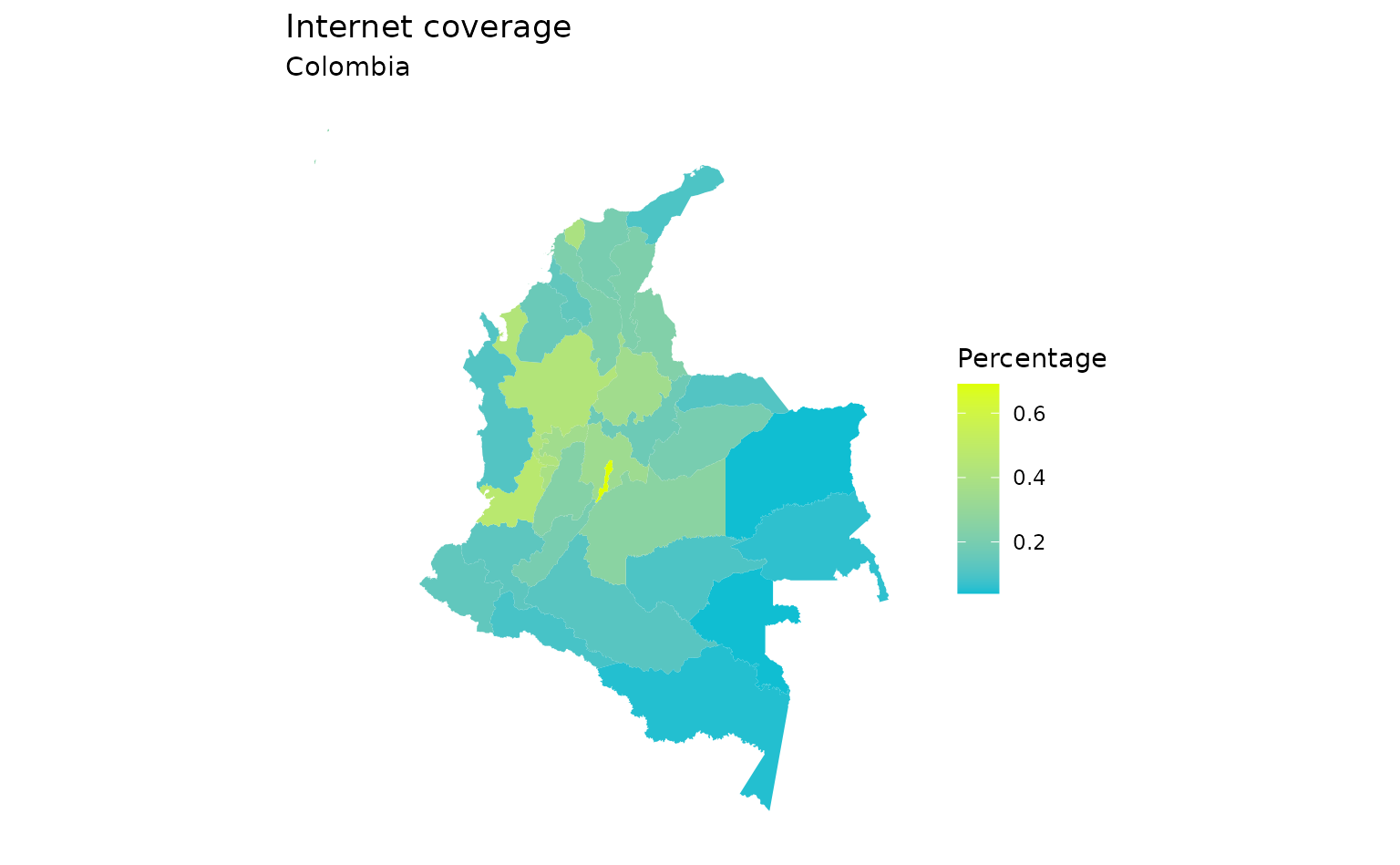
Static plots (ggplot2)
ggplot2 can
be used to generate static plots of spatial data by using the geometry
geom_sf(). Color palettes and themes can be defined for
each plot using the aesthetic and scales, which can be consulted in the
ggplot2 documentation.
We will use a gradient with a two-color diverging palette, to make the
differences more visible.
ggplot(data = internet_cov) +
  geom_sf(mapping = aes(fill = internet), color = NA) +
  theme_minimal() +
  theme(
    plot.background = element_rect(fill = "white", colour = "white"),
    panel.background = element_rect(fill = "white", colour = "white"),
    panel.grid = element_blank(),
    axis.text = element_blank(),
    axis.ticks = element_blank()
  ) +
  scale_fill_gradient("Percentage", low = "#10bed2", high = "#deff00") +
  ggtitle(
    label = "Internet coverage",
    subtitle = "Colombia"
  )
Dynamic plots (leaflet)
For dynamic plots, we can use leaflet,
which is an open-source library for interactive maps. To create the same
plot we first will create the color palette.
colfunc <- colorRampPalette(c("#10bed2", "#deff00"))
pal <- colorNumeric(
  palette = colfunc(100),
  domain = internet_cov[["internet"]]
)
With the previous color palette we can generate the interactive plot.
The package also includes open source maps for the base map like OpenStreetMap
and CartoDB. For further
details on leaflet, please refer to the package’s documentation.
leaflet(internet_cov) %>%
  addProviderTiles(providers$CartoDB.Positron) %>%
  addPolygons(
    stroke = TRUE,
    weight = 0,
    color = NA,
    fillColor = ~ pal(internet_cov[["internet"]]),
    fillOpacity = 1,
    popup = paste0(internet_cov[["internet"]])
  ) %>%
  addLegend(
    position = "bottomright",
    pal = pal,
    values = ~ internet_cov[["internet"]],
    opacity = 1,
    title = "Internet Coverage"
  )