Population Projections with ColOpenData
Source:vignettes/population_projections.Rmd
population_projections.RmdWe can use ColOpenData to retrieve population projections and back-projections on multiple levels of spatial aggregation, including municipalities, departments and national levels. Availability of years depends on spatial levels. These projections include differentiation by gender and even ethnic groups; however, the latter is only available for municipalities.
Availability of years by spatial levels goes as follows:
| Level | Years |
|---|---|
| National | 1950 - 2070 |
| National with sex | 1985 - 2050 |
| Department | 1985 - 2050 |
| Department with Sex | 1985 - 2050 |
| Municipality | 1985 - 2035 |
| Municipality with Sex | 1985 - 2035 |
| Municipaity with Sex and Ethnic Groups | 2018 - 2035 |
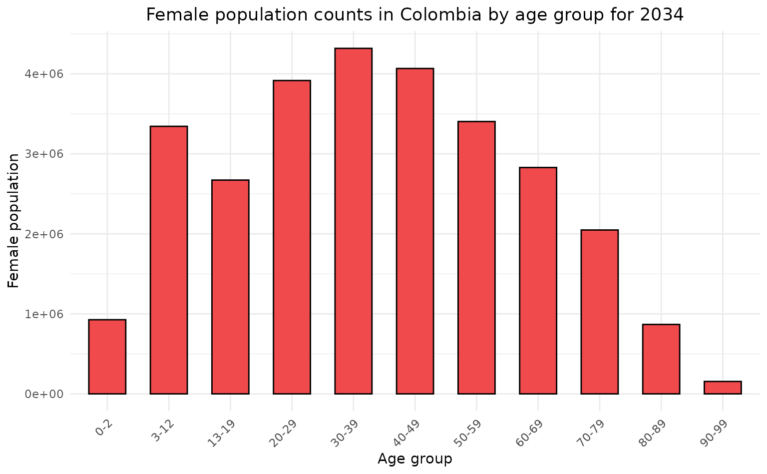
For this example, we will present projections and back projections of national population by area, sex and age for the period from 1950 to 2070. We will observe the expected female population under 99 by personalized age brackets for 2034.
We will first load the needed libraries.
library(ColOpenData)
library(dplyr)
#>
#> Attaching package: 'dplyr'
#> The following objects are masked from 'package:stats':
#>
#>     filter, lag
#> The following objects are masked from 'package:base':
#>
#>     intersect, setdiff, setequal, union
library(ggplot2)
Now we can download the data. We will use the function
download_pop_projections(), which has five parameters:
-
spatial_levelcharacter with the spatial level to be consulted. Can be either"national","department"or"municipality". -
start_yearnumeric with the start year to be consulted. -
end_yearnumeric with the end year to be consulted. -
include_sexlogical for including (or not) division by sex. Default isFALSE. -
include_ethniclogical for including (or not) division by ethnic group (only available for"municipality"). Default isFALSE.
asen <- download_pop_projections(
  spatial_level = "national",
  start_year = 2034,
  end_year = 2034,
  include_sex = TRUE,
  include_ethnic = FALSE
)
#> ColOpenData provides open data derived from Departamento Administrativo
#> Nacional de Estadística (DANE), and Instituto de Hidrología,
#> Meteorología y Estudios Ambientales (IDEAM) but with modifications for
#> specific functional needs. These changes may alter the structure,
#> format, or content, meaning the data does not reflect the official
#> dataset. The package is developed independently, with no endorsement or
#> involvement from these institutions or any Colombian government body.
#> The authors of ColOpenData are not liable for how users utilize the
#> data, and users are responsible for any outcomes from their use or
#> analysis of the data.
#> Stored by Universidad de Los Andes under the Epiverse TRACE initiative.
We will filter the downloaded data for ages under 99.
female_2034 <- asen %>%
  filter(
    area == "total",
    sexo == "mujer",
    edad != "100_y_mas"
  ) %>%
  mutate(edad = as.numeric(edad))
Age groups will be defined by breaks and included in the original dataset.
age_groups <- cut(female_2034[["edad"]],
  breaks = c(-1, 2, 12, 19, 29, 39, 49, 59, 69, 79, 89, 99),
  labels = c(
    "0-2", "3-12", "13-19", "20-29", "30-39", "40-49",
    "50-59", "60-69", "70-79", "80-89", "90-99"
  )
)
female_groups <- female_2034 %>%
  mutate(age_group = age_groups) %>%
  group_by(age_group) %>%
  summarise(total_sum = sum(total))
Finally, we can plot the output.
ggplot(female_groups, aes(
  x = age_group,
  y = total_sum
)) +
  geom_bar(stat = "identity", fill = "#f04a4c", color = "black", width = 0.6) +
  labs(
    title = "Female population counts in Colombia by age group for 2034",
    x = "Age group",
    y = "Female population"
  ) +
  theme_minimal() +
  theme(
    plot.background = element_rect(fill = "white", colour = "white"),
    panel.background = element_rect(fill = "white", colour = "white"),
    axis.text.x = element_text(angle = 45, hjust = 1),
    plot.title = element_text(hjust = 0.5)
  )