A Deep Dive into Colombian Demographics Using ColOpenData
Source:vignettes/demographic_data.Rmd
demographic_data.RmdColOpenData can be used to access open demographic data from Colombia. This demographic data is retrieved from Departamento Administrativo Nacional de Estadística (DANE). The demographic module allows you to consult demographic data from the National Population and Dwelling Census (CNPV) of 2018 and Population Projections.
The available CNPV information is divided in four categories: households, persons demographic, persons social and dwellings. The population projections information presents data from 1950 to 2070 for a national level, from 1985 to 2050 for a departmental level and from 1985 to 2035 for a municipal level. All data documentation can be accessed as explained at Documentation and Dictionaries.
In this vignette you will learn:
- How to download demographic data using ColOpenData.
- How to filter, group, mutate and aggregate demographic data.
- How to visualize data using ggplot2.
As the goal of this vignette is to show some examples on how to use the data, we will load some specific libraries but that does not mean they are required to use the data in all cases.
In order to access its documentation we need to use the function
list_datasets() and indicate as a parameter the module we
are interested in. It is important to take a good look at this to have a
clearer understanding of what we count with, before just throwing
ourselves to work with the data. Now, we should start by loading all
necessary libraries.
Disclaimer: all data is loaded to the environment in the user’s R session, but is not downloaded to user’s computer.
Initial Exploration: Basic Data Handling with ColOpenData
Documentation access
First, we have to access the demographic documentation, to check available datasets.
datasets_dem <- list_datasets(module = "demographic", language = "EN")

head(datasets_dem)
#> # A tibble: 6 × 7
#>   name                group       source year  level        category description
#>   <chr>               <chr>       <chr>  <chr> <chr>        <chr>    <chr>
#> 1 DANE_CNPVH_2018_1HD demographic DANE   2018  department   househo… Number of …
#> 2 DANE_CNPVH_2018_1HM demographic DANE   2018  municipality househo… Number of …
#> 3 DANE_CNPVH_2018_2HD demographic DANE   2018  department   househo… Number of …
#> 4 DANE_CNPVH_2018_2HM demographic DANE   2018  municipality househo… Number of …
#> 5 DANE_CNPVH_2018_3HD demographic DANE   2018  department   househo… Households…
#> 6 DANE_CNPVH_2018_3HM demographic DANE   2018  municipality househo… Households…
After checking the documentation, we can load the data we want to
work with. To do this, we will use the
download_demographic() function that takes by parameter the
dataset name, presented in the documentation. For this first example we
will focus on a CNPV dataset.
Data load
public_services_d <- download_demographic(dataset = "DANE_CNPVV_2018_8VD")
#> ColOpenData provides open data derived from Departamento Administrativo
#> Nacional de Estadística (DANE), and Instituto de Hidrología,
#> Meteorología y Estudios Ambientales (IDEAM) but with modifications for
#> specific functional needs. These changes may alter the structure,
#> format, or content, meaning the data does not reflect the official
#> dataset. The package is developed independently, with no endorsement or
#> involvement from these institutions or any Colombian government body.
#> The authors of ColOpenData are not liable for how users utilize the
#> data, and users areresponsible for any outcomes from their use or
#> analysis of the data.
#> Stored by Universidad de Los Andes under the Epiverse TRACE iniative.
head(public_services_d)
#> codigo_departamento departamento area servicio_publico disponible
#> 1 00 Total nacional total energia_electrica si
#> 2 00 Total nacional total energia_electrica no
#> 3 00 Total nacional total energia_electrica sin_informacion
#> 4 00 Total nacional cabecera energia_electrica si
#> 5 00 Total nacional cabecera energia_electrica no
#> 6 00 Total nacional cabecera energia_electrica sin_informacion
#> total
#> 1 12984126
#> 2 496603
#> 3 0
#> 4 10485896
#> 5 81579
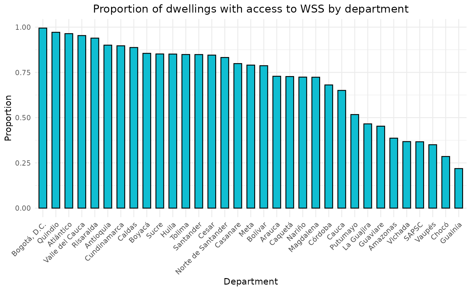
#> 6 0As it can be seen above, public_services_d presents information regarding availability of public services in the country at the department level. Now, with this data we could, for example, find the proportion of dwellings that have access to a water supply system (WSS) by department and plot it.
Data filter and plot
First we will subset the data so it presents the information regarding the WSS by department.
wss <- public_services_d %>%
  filter(
    area == "total_departamental",
    servicio_publico == "acueducto"
  ) %>%
  select(departamento, disponible, total)
With the subset, we can calculate the total counts by department.
Then, we can calculate the proportions of “yes” (“si”) by department.
proportions_wss <- wss %>%
  filter(disponible == "si") %>%
  left_join(total_counts, by = "departamento") %>%
  mutate(proportion_si = total / total_all)
For plotting purposes, we will change the name of “San Andrés”, since the complete name is too long.
proportions_wss[28, "departamento"] <- "SAPSC"Finally, we can plot the results
ggplot(proportions_wss, aes(
  x = reorder(departamento, -proportion_si),
  y = proportion_si
)) +
  geom_bar(stat = "identity", fill = "#10bed2", color = "black", width = 0.6) +
  labs(
    title = "Proportion of dwellings with access to WSS by department",
    x = "Department",
    y = "Proportion"
  ) +
  theme_minimal() +
  theme(
    plot.background = element_rect(fill = "white", colour = "white"),
    panel.background = element_rect(fill = "white", colour = "white"),
    axis.text.x = element_text(angle = 45, hjust = 1),
    plot.title = element_text(hjust = 0.5)
  )