ColOpenData can be used to access open climate data from Colombia. This climate data is retrieved from Instituto de Hidrología, Meteorología y Estudios Ambientales (IDEAM). The climate module allows the user to consult climate data for any Region of Interest (ROI) inside the country and retrieve the information for each station contained inside.
The available information from IDEAM can be accessed using specific internal tags as follows:
| Tags | Variable |
|---|---|
| TSSM_CON | Dry-bulb Temperature |
| THSM_CON | Wet-bulb Temperature |
| TMN_CON | Minimum Temperature |
| TMX_CON | Maximum Temperature |
| TSTG_CON | Dry-bulb Temperature (Termograph) |
| HR_CAL | Relative Humidity |
| HRHG_CON | Relative Humidity (Hydrograph) |
| TV_CAL | Vapour Pressure |
| TPR_CAL | Dew Point |
| PTPM_CON | Precipitation (Daily) |
| PTPG_CON | Precipitation (Hourly) |
| EVTE_CON | Evaporation |
| FA_CON | Atmospheric Phenomenon |
| NB_CON | Cloudiness |
| RCAM_CON | Wind Trajectory |
| BSHG_CON | Sunshine Duration |
| VVAG_CON | Wind Speed |
| DVAG_CON | Wind Direction |
| VVMXAG_CON | Maximum Wind Speed |
| DVMXAG_CON | Maximum Wind Direction |
Each observation is subject to the availability of stations in the ROI and the stations’ status (active, maintenance or suspended), as well as quality filters implemented by IDEAM.
In this vignette you will learn:
- How to download climate data using ColOpenData.
- How to aggregate climate data by different frequencies
- How to plot downloaded climate data
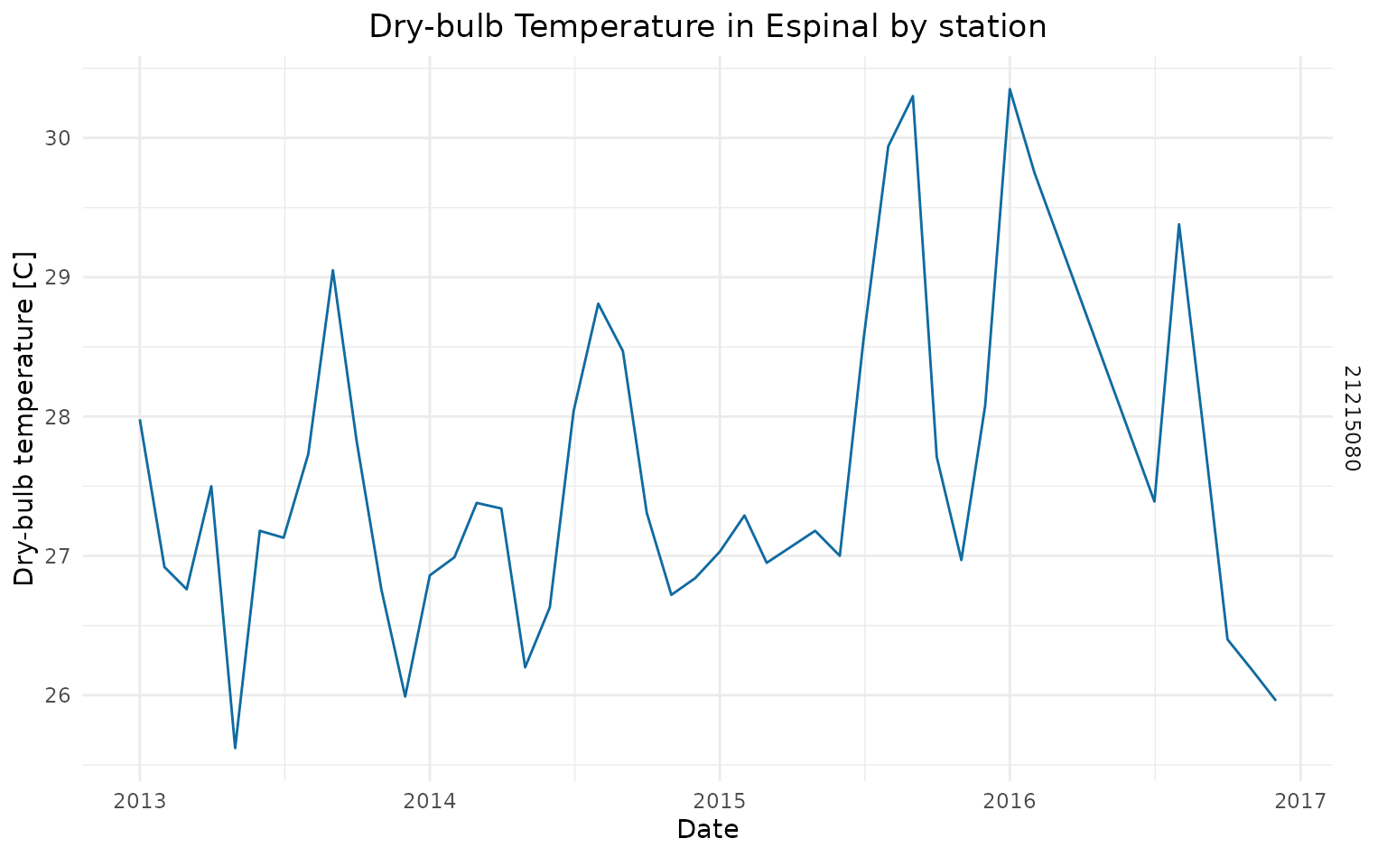
For this example we will retrieve data for the municipality of Espinal in Colombia. We will download Dry-Bulb Temperature (TSSM_CON) from 2013 to 2016, to observe the increase in the average temperature during 2015 and 2016 due to the impact of El Nino (ENSO).
ColOpenData offers three methods to do this, using
different functions: - download_climate_stations() to
download climate data from previously selected stations -
download_climate_geom() to download climate data from a
specified geometry (ROI) - download_climate() to download
climate data from municipalities’ or departments’ already loaded
geometries
In this example, we will follow the three methods to get the same results, exploring the included functions. We will start by loading the needed libraries.
Disclaimer: all data is loaded to the environment in the user’s R session, but is not downloaded to user’s computer.
Retrieving climate data for a ROI using stations’ data
For this example, we will need to create a spatial polygon around the
municipality of Espinal and use that as our ROI to retrieve the climate
data. To create the spatial polygon we need to introduce the coordinates
of the geometry. For simplicity, we will build a bounding box by
introducing the 4 points which bound the municipality, and transform the
created geometry into an sf object (see sf
library for further details).
lat <- c(4.263744, 4.263744, 4.078156, 4.078156, 4.263744)
lon <- c(-75.042067, -74.777022, -74.777022, -75.042067, -75.042067)
polygon <- st_polygon(x = list(cbind(lon, lat))) %>% st_sfc()
roi <- st_as_sf(polygon)
With our created ROI, we can make a simple visualization using
leaflet.
leaflet(roi) %>%
  addProviderTiles("OpenStreetMap") %>%
  addPolygons(
    stroke = TRUE,
    weight = 2,
    color = "#2e6930",
    fillColor = "#2e6930",
    opacity = 0.6
  )
We can make a first exploration to check if there are any stations
contained inside of it, using the function
stations_in_roi().
stations <- stations_in_roi(geometry = roi)

head(stations)
#> Simple feature collection with 6 features and 20 fields
#> Geometry type: POINT
#> Dimension:     XY
#> Bounding box:  xmin: -75 ymin: 4.15 xmax: -74.78361 ymax: 4.258278
#> CRS:           NA
#>        codigo                      nombre           categoria
#> 78   21185090    NATAIMA - AUT [21185090]   Agrometeorológica
#> 1544 21170020    DOS AGUAS LAS [21170020]       Pluviométrica
#> 1692 21180220 AEROPUERTO FARCA [21180220]       Pluviométrica
#> 1929 21180230  BAMBU EL MOLINO [21180230]       Pluviométrica
#> 1935 21215090        MARANONES [21215090] Climática Ordinaria
#> 2084 21215080         CHICORAL [21215080] Climática Ordinaria
#>                     tecnologia     estado departamento       municipio
#> 78   Automática con Telemetría     Activa       Tolima         Espinal
#> 1544              Convencional     Activa       Tolima Suárez (Tolima)
#> 1692              Convencional Suspendida       Tolima         Espinal
#> 1929              Convencional Suspendida       Tolima         Espinal
#> 1935              Convencional Suspendida       Tolima         Espinal
#> 2084              Convencional     Activa       Tolima         Espinal
#>         latitud     longitud altitud fecha_instalacion
#> 78   4.18813889 -74.96047222     393        2005-10-16
#> 1544 4.25827778 -74.78361111    3394        1951-01-15
#> 1692       4.15        -74.9     350        1979-11-15
#> 1929        4.2        -75.0     390        1979-11-15
#> 1935 4.21666667 -74.93333333     370        1959-06-15
#> 2084 4.23152778 -74.99536111     432        1963-05-15
#>                  area_operativa   corriente area_hidrografica zona_hidrografica
#> 78   Area Operativa 10 - Tolima      Cuinde   Magdalena Cauca    Alto Magdalena
#> 1544 Area Operativa 10 - Tolima      Coello   Magdalena Cauca    Alto Magdalena
#> 1692 Area Operativa 10 - Tolima       Tuamo   Magdalena Cauca    Alto Magdalena
#> 1929 Area Operativa 10 - Tolima Rio Salinas   Magdalena Cauca    Alto Magdalena
#> 1935 Area Operativa 10 - Tolima      Blanco   Magdalena Cauca    Alto Magdalena
#> 2084 Area Operativa 10 - Tolima       Luisa   Magdalena Cauca    Alto Magdalena
#>                                 subzona_hidrografica
#> 78           Río Luisa y otros directos al Magdalena
#> 1544 Directos Magdalena entre ríos Cabrera y Sumapaz
#> 1692         Río Luisa y otros directos al Magdalena
#> 1929         Río Luisa y otros directos al Magdalena
#> 1935                                      Río Coello
#> 2084                                      Río Coello
#>                                                          entidad
#> 78   INSTITUTO DE HIDROLOGIA METEOROLOGIA Y ESTUDIOS AMBIENTALES
#> 1544 INSTITUTO DE HIDROLOGIA METEOROLOGIA Y ESTUDIOS AMBIENTALES
#> 1692 INSTITUTO DE HIDROLOGIA METEOROLOGIA Y ESTUDIOS AMBIENTALES
#> 1929 INSTITUTO DE HIDROLOGIA METEOROLOGIA Y ESTUDIOS AMBIENTALES
#> 1935 INSTITUTO DE HIDROLOGIA METEOROLOGIA Y ESTUDIOS AMBIENTALES
#> 2084 INSTITUTO DE HIDROLOGIA METEOROLOGIA Y ESTUDIOS AMBIENTALES
#>      fecha_suspension codigo_municipio codigo_departamento
#> 78               <NA>            73268                  73
#> 1544             <NA>            73770                  73
#> 1692       2000-04-15            73268                  73
#> 1929       1984-10-15            73319                  73
#> 1935       1971-08-15            73200                  73
#> 2084             <NA>            73268                  73
#>                        geometry
#> 78   POINT (-74.96047 4.188139)
#> 1544 POINT (-74.78361 4.258278)
#> 1692         POINT (-74.9 4.15)
#> 1929            POINT (-75 4.2)
#> 1935 POINT (-74.93333 4.216667)
#> 2084 POINT (-74.99536 4.231528)
We can see that in the region there are 24 stations. Different categories are recorded by different stations, and can be checked at the column categoria. Stations under the categories Climática Principal and Climática Ordinaria have records of temperature.
Some stations are suspended, which means they are not taking
measurements at the moment. This information is found at the column
estado where, if suspended, the observation would be
Suspendida Also, at the column fecha_suspension the
observation would be different from NA, since suspended
stations would have an associated suspension date. However, even if a
station is suspended, the historical data (up to the suspension date)
can be accessed.
To filter the stations that recorded information during the desired period, we can delete the stations with suspension dates before 2013.
cw_stations <- stations %>%
  filter(
    as.Date(fecha_suspension) > as.Date("2013-01-01") | estado == "Activa",
    categoria %in% c("Climática Principal", "Climática Ordinaria")
  )

head(cw_stations)
#> Simple feature collection with 1 feature and 20 fields
#> Geometry type: POINT
#> Dimension:     XY
#> Bounding box:  xmin: -74.99536 ymin: 4.231528 xmax: -74.99536 ymax: 4.231528
#> CRS:           NA
#>     codigo              nombre           categoria   tecnologia estado
#> 1 21215080 CHICORAL [21215080] Climática Ordinaria Convencional Activa
#>   departamento municipio    latitud     longitud altitud fecha_instalacion
#> 1       Tolima   Espinal 4.23152778 -74.99536111     432        1963-05-15
#>               area_operativa corriente area_hidrografica zona_hidrografica
#> 1 Area Operativa 10 - Tolima     Luisa   Magdalena Cauca    Alto Magdalena
#>   subzona_hidrografica
#> 1           Río Coello
#>                                                       entidad fecha_suspension
#> 1 INSTITUTO DE HIDROLOGIA METEOROLOGIA Y ESTUDIOS AMBIENTALES             <NA>
#>   codigo_municipio codigo_departamento                   geometry
#> 1            73268                  73 POINT (-74.99536 4.231528)
From the original 24 stations, only 1 was working for some or the whole period of interest and collected information for Dry-Bulb Temperature (TSSM_CON). It is important to consider that after data collection, some information might be lost due to quality attributes.
With the stations, we can access TMX_CON from 2013 to 2016. To do so,
we can use the function download_climate_stations(). This
function has the following parameters:
-
stations:data.framecontaining the stations’ codes. Thisdata.framemust be retrieved from the functionstations_in_roi. -
start_date: character with the first date to consult in the format"YYYY-MM-DD". (First available date is"1920-01-01"). -
end_date: character with the last date to consult in the format"YYYY-MM_DD". (Last available date is"2023-05-31"). -
tag: character containing climate tag to consult.
tssm_stations <- download_climate_stations(
  stations = cw_stations,
  start_date = "2013-01-01",
  end_date = "2016-12-31",
  tag = "TSSM_CON"
)
#> ColOpenData provides open data derived from Departamento Administrativo
#> Nacional de Estadística (DANE), and Instituto de Hidrología,
#> Meteorología y Estudios Ambientales (IDEAM) but with modifications for
#> specific functional needs. These changes may alter the structure,
#> format, or content, meaning the data does not reflect the official
#> dataset. The package is developed independently, with no endorsement or
#> involvement from these institutions or any Colombian government body.
#> The authors of ColOpenData are not liable for how users utilize the
#> data, and users are responsible for any outcomes from their use or
#> analysis of the data.
#> Stored by Universidad de Los Andes under the Epiverse TRACE initiative.

head(tssm_stations)
#>    station    longitude   latitude       date     hour      tag value
#> 1 21215080 -74.99536111 4.23152778 2013-01-01 07:00:00 TSSM_CON  23.2
#> 2 21215080 -74.99536111 4.23152778 2013-01-01 13:00:00 TSSM_CON  32.0
#> 3 21215080 -74.99536111 4.23152778 2013-01-01 18:00:00 TSSM_CON  27.2
#> 4 21215080 -74.99536111 4.23152778 2013-01-02 07:00:00 TSSM_CON  22.6
#> 5 21215080 -74.99536111 4.23152778 2013-01-02 13:00:00 TSSM_CON  32.0
#> 6 21215080 -74.99536111 4.23152778 2013-01-02 18:00:00 TSSM_CON  27.0
The returned tidy data.frame includes: individual and
unique station code, longitude, latitude, date, hour, tag requested and
value recorded at the specified time. The tidy structure reports a row
for each observation, which makes the subset and plot easier.
To plot a time series of the stations’ data we can use
ggplot() function from ggplot2 package as
follows:
ggplot(data = tssm_stations) +
  geom_line(aes(x = date, y = value, group = station), color = "#106ba0") +
  ggtitle("Dry-bulb Temperature in Espinal by station") +
  xlab("Date") +
  ylab("Temperature [°C]") +
  facet_grid(rows = vars(station)) +
  theme_minimal() +
  theme(
    plot.background = element_rect(fill = "white", colour = "white"),
    panel.background = element_rect(fill = "white", colour = "white"),
    plot.title = element_text(hjust = 0.5)
  )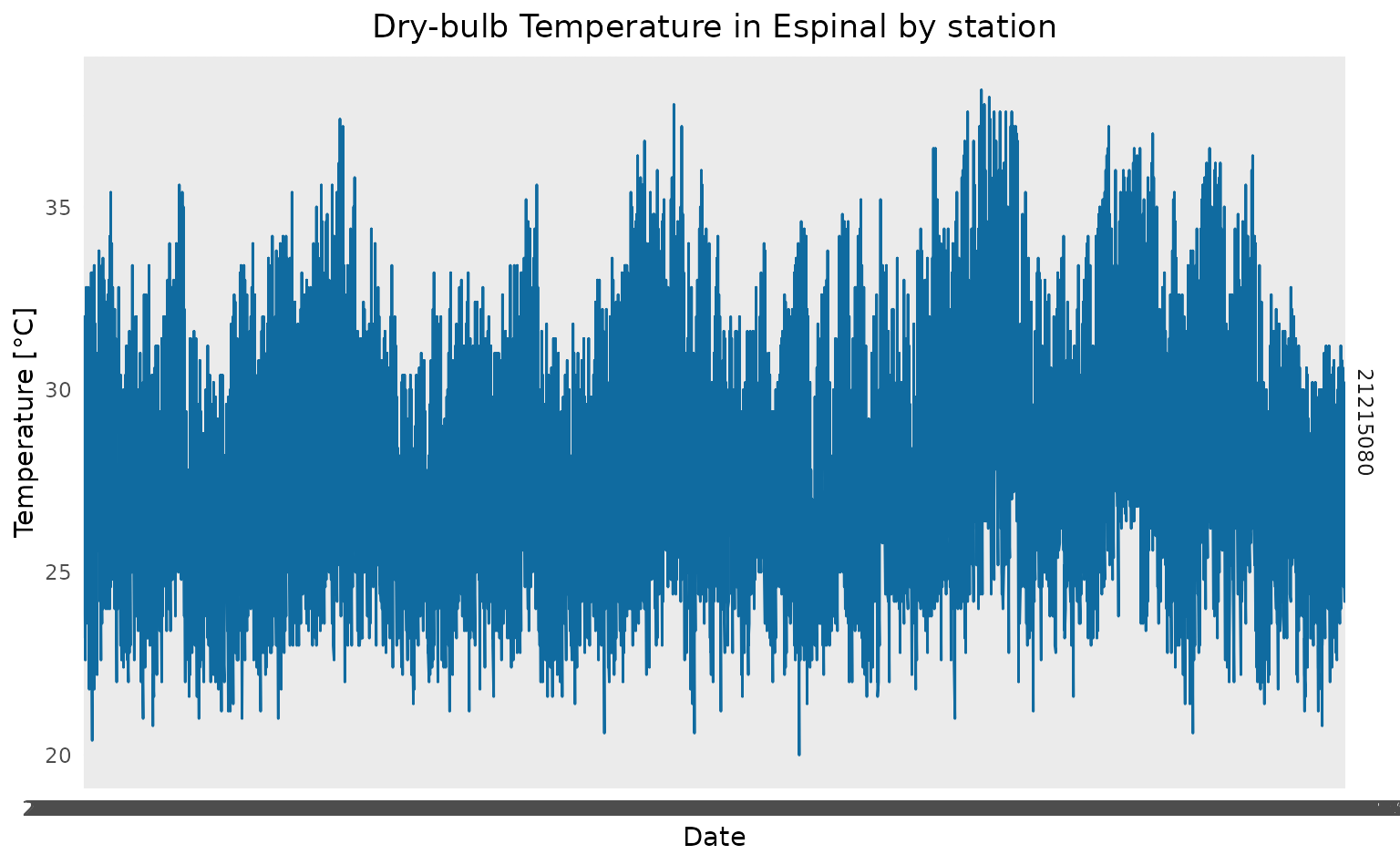
As we can see, only one station has data for the selected period.
However, by having the data measured by hours, we cannot easily observe
changes in the temperature patterns along time. To aid this issue, we
will use the aggregation function aggregate_climate(),
which aggregates climate data by time. This function takes by parameter
the desired aggregation.
tssm_month <- tssm_stations %>% aggregate_climate(frequency = "month")

ggplot(data = tssm_month) +
  geom_line(aes(x = date, y = value, group = station), color = "#106ba0") +
  ggtitle("Dry-bulb Temperature in Espinal by station") +
  xlab("Date") +
  ylab("Dry-bulb temperature [C]") +
  facet_grid(rows = vars(station)) +
  theme_minimal() +
  theme(
    plot.background = element_rect(fill = "white", colour = "white"),
    panel.background = element_rect(fill = "white", colour = "white"),
    plot.title = element_text(hjust = 0.5)
  )
## Other methods ::: {style=“text-align: justify;”} To retrieve climate
data for any ROI in the country, without manually extracting the
stations’ data, we can use the function
## Other methods ::: {style=“text-align: justify;”} To retrieve climate
data for any ROI in the country, without manually extracting the
stations’ data, we can use the function
download_climate_geom(). The function has the following
parameters:
-
geometry:sfgeometry containing the geometry for a given ROI. This geometry can be either aPOLYGONorMULTIPOLYGON. -
start_date: character with the first date to consult in the format"YYYY-MM-DD". (First available date is"1920-01-01"). -
end_date: character with the last date to consult in the format"YYYY-MM_DD". (Last available date is"2023-05-31"). -
tag: character containing climate tag to consult.
To replicate the previous example, we can just use the previously
created ROI and add the aggregation for month. We can add the
aggregation function to the workflow using the pipe operator
%>%. The following code should retrieve the same results
as the previous one. :::
tssm_roi <- download_climate_geom(
  geometry = roi,
  start_date = "2013-01-01",
  end_date = "2016-12-31",
  tag = "TSSM_CON"
) %>% aggregate_climate(frequency = "month")
To make the download process even easier, and avoid the creation of already known geometries like municipalities or departments, ColOpenData offers an extra function to download data using the areas’ DIVIPOLA code.
DIVIPOLA codification is standardized for the whole country, and contains departments’ and municipalities’ codes. For further details on DIVIPOLA codification and functions please refer to Documentation and Dictionaries. We will filter for the city of Espinal in the department Tolima. :::
espinal_code <- name_to_code_mun("Tolima", "Espinal")
espinal_code
#> [1] "73268"
The function download_climate() will require almost the
same arguments as download_climate_geom(), but instead of
an sf object, it will take a character containing the
DIVIPOLA code:
-
code: character with the DIVIPOLA code for the area. -
start_date: character with the first date to consult in the format"YYYY-MM-DD". (First available date is"1920-01-01"). -
end_date: character with the last date to consult in the format"YYYY-MM_DD". (Last available date is"2023-05-31"). -
tag: character containing climate tag to consult.
The code below can be used to get the same results as the previous two examples, without the need to create a whole geometry or filtering individual stations.
tssm_mpio <- download_climate(
  code = espinal_code,
  start_date = "2013-01-01",
  end_date = "2016-12-31",
  tag = "TMX_CON"
) %>% aggregate_climate(frequency = "month")
Disclaimer
Data availability is subdued to station’s measurements and quality filters. In most cases, this leads to a lower amount of data, considering the extensive amount of climate stations.
-
Temporal aggregation is only available for some tags and is limited to the ones who have a specific methodology of aggregation reported by IDEAM. The daily, monthly and annual aggregation is available for:
-
TSSM_CON: Dry-bulb temperature -
TMX_CON: Maximum temperature -
TMN_CON: Minimum temperature -
PTPM_CON: Precipitation -
BSHG_CON: Sunshine duration
-
Temporal and spatial interpolation are not included in this version of ColOpenData.