Simulate transmission chains
Last updated on 2026-07-17 | Edit this page
Estimated time: 32 minutes
Overview
Questions
- How can we simulate transmission chains based on infection characteristics?
Objectives
- Estimate the potential for large outbreaks following the introduction of a new case using a branching process with epichains.
Prerequisites
Learners should familiarise themselves with the following concept dependencies before working through this tutorial:
Statistics: Common probability distributions, including Poisson and negative binomial.
Epidemic theory: The reproduction number, \(R\).
R packages installed: epichains, epiparameter, tidyverse.
Install packages if they are not already installed
R
if (!base::require("pak")) install.packages("pak")
pak::pak(c("epichains", "epiparameter", "tidyverse"))
If you have any error message, go to the main setup page.
Introduction
Individual variation in transmission can affect both the potential for an epidemic to establish in a population and the ease of control (Cori et al., 2017).
Greater variation reduces the overall probably of a single new case causing a large local outbreak, because most cases infect few others and individuals that generate a large number of secondary cases are relatively rare.
However, if a ‘superspreading event’ does occur and the outbreak gets established, this variation can make an outbreak harder to control using mass interventions (i.e. blanket interventions that implicitly assume everyone contributes equally to transmission), because some cases contribute disproportionality: a single uncontrolled case may generate a large number of secondary cases.
Conversely, variation in transmission may provide opportunities for targeted interventions if the individuals who contribute more to transmission (due to biological or behavioural factors), or the settings in which ‘superspreading events’ occur, share socio-demographic, environmental or geographical characteristics that can be defined.
How can we quantify the potential of a new infection to cause a large outbreak based on its reproduction number \(R\) and the dispersion \(k\) of its offspring distribution?
In this episode, we will use the epichains package to simulate transmission chains and estimate the potential for large outbreaks following the introduction of a new case. We are going to use it with functions from epiparameter, dplyr and purrr, so also loading the tidyverse package:
R
library(epichains)
library(epiparameter)
library(tidyverse)
The double-colon
The double-colon :: in R lets you call a specific
function from a package without loading the entire package into the
current environment. The package must be installed.
For example, dplyr::filter(data, condition) uses
filter() from the dplyr package.
This help us remember package functions and avoid namespace conflicts.
Simulation of uncontrolled outbreaks
Infectious disease epidemics spread through populations when a chain of infected individuals transmit the infection to others. Branching processes can be used to model this transmission. A branching process is a stochastic process (i.e. a random process that can be described by a known probability distribution), where each infectious individual gives rise to a random number of individuals in the next generation of infection, starting with the index case in generation 1. The distribution of the number of secondary cases each individual generates is called the offspring distribution (Azam & Funk, 2024).
epichains provides methods to analyse and simulate the size and length of branching processes with an given offspring distribution. epichains implements a rapid and simple model to simulate transmission chains to assess epidemic risk, project cases into the future, and evaluate interventions that change \(R\).
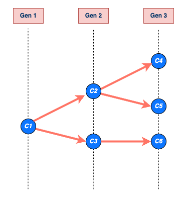
chain size and length
The size of the transmission chain is defined as the total number of individuals infected across all generations of infection, and
the length of the transmission chain is the number of generations from the first case to the last case in the outbreak before the chain ended.
The size calculation includes the first case, and the length calculation contains the first generation when the first case starts the chain (See figure below).
To use epichains, we need to know (or assume) two key epidemiological values:
- the offspring distribution and
- the generation time.
You may recognize these two parameters from the Access epidemiological delay distributions tutorial, where we first introduced generation time and the reproduction number.
Get the offspring distribution
Here we assume the MERS offspring distribution follows a negative
binomial distribution, with mean (reproduction number \(R\)) and dispersion \(k\) values estimated from the linelist and
contact data of mers_korea_2015 in the
outbreaks R package in the previous episode.
R
mers_offspring <- c(mean = 0.60, dispersion = 0.02)
offspring distribution for epichains
We input an offspring distribution to epichains by
referring to the R function that generates random values from the
distribution we want. For a negative binomial distribution, we use
rnbinom with its corresponding mu and
size arguments:
Internally, epichains will draw one random value, given the parameters, to simulate the number of new infections from an infected individual (onward transmission).
R
# generate one random number given the distribution family and its parameters
# (run this line many times to get different values)
rnbinom(n = 1, mu = mers_offspring["mean"], size = mers_offspring["dispersion"])
The reference manual in ?rnbinom tells us our required
specific arguments.
epichains can accept any R function that generates random numbers, so the specified arguments will change depending on the R function used. For more details on the range of possible options, see the function reference manual.
For example, let’s say we want to use a Poisson distribution for the
offspring distribution. First, read the argument required in the
?rpois reference manual. Second, specify the
lambda argument parameter, also known as rate or mean in
the literature. In epichains, this can look like
this:
In this example, we can specify
lambda = mers_offspring["mean"] because the mean number of
secondary cases generated (i.e. \(R\))
should be the same regardless of the distribution we assume. What
changes is the variance of the distribution, and hence the level of
individual-level variation in transmission. When the dispersion
parameter \(k\) approaches infinity
(\(k \rightarrow \infty\)) in a
negative binomial distribution, the variance equals the mean. This makes
the conventional Poisson distribution a special case of the negative
binomial distribution.
Get generation time
The serial interval distribution is often used to approximate the generation time distribution. This approximation is commonly used because it is easier to observe and measure the onset of symptoms in each case than the precise time of infection.
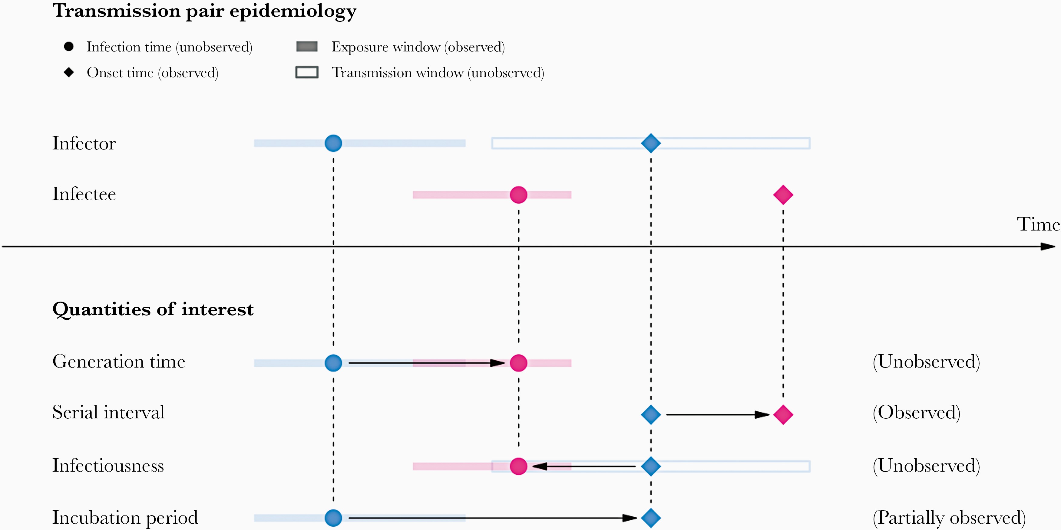
However, using the serial interval as an approximation of the generation time is primarily valid for diseases in which infectiousness starts after symptom onset (Chung Lau et al., 2021). In cases where infectiousness starts before symptom onset, the serial intervals can have negative values, which is the case for diseases with pre-symptomatic transmission (Nishiura et al., 2020).
Let’s use the epiparameter package to access and use the available serial interval for MERS disease.
R
serial_interval <- epiparameter::epiparameter_db(
disease = "mers",
epi_name = "serial",
single_epiparameter = TRUE
)
plot(serial_interval, day_range = 0:25)
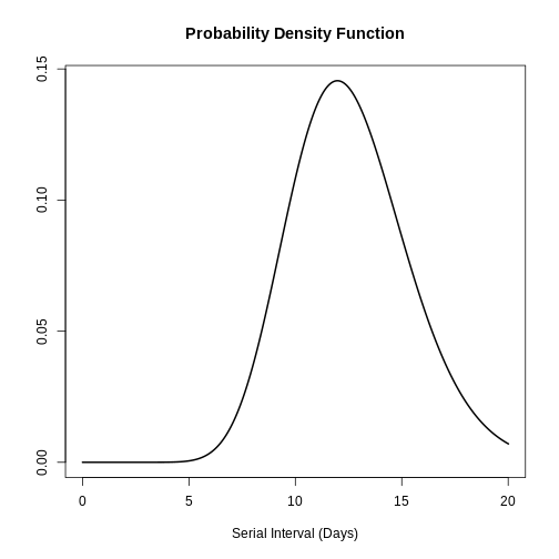
The serial interval for MERS has a mean of 12.6 days and a standard deviation of 2.8 days.
generation time for epichains
In each simulation step, epichains will draw
generation time values for each new infection generated from the
offspring distribution. With <epiparameter> class
objects we can use the distribution function
epiparameter::generate() for this input.
R
# In step one, the number of new infections is 2, then:
# generate 2 random values given the serial interval distribution
generate(x = serial_interval, times = 2)
OUTPUT
[1] 14.60507 15.06471R
# In step two, the number of new infections is 6, then:
# generate 6 random values given the serial interval distribution
generate(x = serial_interval, times = 6)
OUTPUT
[1] 12.522027 16.109812 14.195049 6.875113 15.432142 12.349850Given that the input value in times will vary each step,
we need to embed generate() within a function.
epichains will draw as many random values from the
generation time as number of new infections in that step. This will look
like this:
R
function(x) generate(x = serial_interval, times = x)
This interface is similar to the one cfr uses to link with epiparameter. Read the work with delay distributions vignette for further context.
The function to generate random number from an
<epiparameter> class object can also accept this
notation:
R
as.function(x = serial_interval, func_type = "generate")
Simulate a single chain
Now we are prepared to use the simulate_chains()
function from epichains to create one
transmission chain:
R
epichains::simulate_chains(
n_chains = 1,
statistic = "size",
  offspring_dist = rnbinom,
  mu = mers_offspring["mean"],
  size = mers_offspring["dispersion"],
generation_time = function(x) generate(x = serial_interval, times = x)
)
simulate_chains() requires three sets of arguments as a
minimum:
-
simulation controls (
n_chainsandstatistic), -
offspring distribution (
offspring_distand required distribution parameters), and -
generation time
(
generation_time).
In the lines above, we described how to specify the offspring distribution and generation time. The simulation controls include at least two arguments:
-
n_chains, which defines the number of transmission chains to simulate for and -
statistic, which defines a chain statistic to track (either"size"or"length") as the stopping criteria for each chain being simulated.
Stopping criteria
This is an customisable feature of epichains. By
default, branching process simulations end when they have gone extinct.
For long-lasting transmission chains, in simulate_chains()
you can add the stat_threshold argument.
For example, if we set an stopping criteria for
statistic = "size" of stat_threshold = 500, no
more offspring will be produced after a chain of size 500.
The simulate_chains() output creates a
<epichains> class object, which we can then analyse
further in R.
Simulate multiple chains
We can use simulate_chains() to create multiple chains
and increase the probability of simulating uncontrolled outbreak
projections given an overdispersed offspring distribution.
We need to specify one additional element:
-
set.seed(<integer>)is a function used to initialise a pseudo-random number generator. By specifying a seed value (the<integer>), you ensure that the sequence of numbers produced by subsequent random functions, likernorm()orsimulate_chains(), is identical every time the code is executed.
With this configuration, each chain will represent
one initial case. These cases per chain are
independent, isolated, and without interactions. This means that each
chain will have their own pool of susceptibles, which you can configure
by using the pop or percent_immune
arguments.
Now, let’s simulate 100 transmission chains:
R
# Run all this chunk together to let set.seed() work!
# Set seed for random number generator
set.seed(33)
multiple_epichains <- epichains::simulate_chains(
  n_chains = 100,
  statistic = "size",
  offspring_dist = rnbinom,
  mu = mers_offspring["mean"],
  size = mers_offspring["dispersion"],
  generation_time = function(x) generate(x = serial_interval, times = x)
)
You can inspect the total size of each simulated
chain, equivalent to the cumulative number of cases per chain, using the
summary() to the <epichains> class
object:
R
summary(multiple_epichains)
OUTPUT
`epichains_summary` object

  [1]   1   1   1   1   1   1   1   1   1   1   1   1   1   1   1   1   1   1
 [19]   7   1   1   1   1   1   1   1   1   1   1  14   1   2   1   1   2   1
 [37]   1   1   1   1   1   1   1   1   1   1   1   1   1   1   1   1   1   1
 [55]   1   1   1   1 512   1   1   1   1   1 104   1   1   1   1   1   1   1
 [73]   1   1   1   1   1   1   1   1   1   4   1   1   1   1   1   1   1   1
 [91]   1   1   1   1   1   1   1   1   1   1

 Simulated sizes:

Max: 512
Min: 1
We can visually count how many chains reach to more than 100 infected cases, with the maximum and minimun counts too.
Challenge
Use the last run of epichains::simulate_chains() for
simulating multiple chains. Change the statistic from
"size" to "length". Run the
summary() function.
- What chain feature does this output show?
If you need help, return to the “Chain size and length” callout box from the beginning.
Read the epichains output
To explore the output format of the <epichains>
class object of name multiple_epichains, let’s look at the
simulated chain number 30.
Let’s use dplyr::filter() for this:
R
chain_to_observe <- 30
R
#### get epichain summary ----------------------------------------------------

multiple_epichains %>%
  dplyr::filter(chain == chain_to_observe)
OUTPUT
`<epichains>` object

< epichains head (from first known infector) >

  chain infector infectee generation      time
2    30        1        2          2 14.100967
3    30        1        3          2 10.640301
4    30        1        4          2 15.608764
5    30        1        5          2 13.515424
6    30        1        6          2  9.967474
7    30        1        7          2  9.376222


Number of chains: 100
Number of infectors (known): 3
Number of generations: 3
Use `as.data.frame(<object_name>)` to view the full output in the console.
This output contains two parts:
- A
head()print of the infector-infectee pairs starting from the first known infector. - A summary footer, the piece of text that appears at the bottom:
OUTPUT
Number of infectors (known): 3
Number of generations: 3
The simulated chain number 30 has three known infectors
and three generations. These numbers are more visible when printing the
<epichains> objects as a data frame (or
<tibble>).
R
#### infector-infectee data frame --------------------------------------------

multiple_epichains %>%
  dplyr::filter(chain == chain_to_observe) %>%
  dplyr::as_tibble()
OUTPUT
# A tibble: 14 × 5
   chain infector infectee generation  time
   <int>    <dbl>    <dbl>      <int> <dbl>
 1    30       NA        1          1  0
 2    30        1        2          2 14.1
 3    30        1        3          2 10.6
 4    30        1        4          2 15.6
 5    30        1        5          2 13.5
 6    30        1        6          2  9.97
 7    30        1        7          2  9.38
 8    30        1        8          2 11.5
 9    30        4        9          3 31.0
10    30        4       10          3 25.3
11    30        4       11          3 28.5
12    30        4       12          3 29.6
13    30        4       13          3 25.9
14    30        4       14          3 24.6
Chain 30 tells us a story:
“In the first transmission generation at time = 0, one
subject (ID = NA) infected the subject with
ID = 1. Subject ID = 1 is the first known
infector.
“Then, in the second transmission generation, subject
ID = 1 infected seven subjects, from ID = 2 to
ID = 8. These infections ocurred in time
between day 9 and day 15, after the first known infection.
“Later, in the third transmission generation, subject
ID = 4 infected six new subjects, from ID = 9
to ID = 14. These infections ocurred in time
between day 24 and day 31, after the first known infection.”
The output data frame collects infectees as the observation unit:
- Each infectee has a
infectee“ID”. - Each infectee that behaved as an infector is
registered in the
infectorcolumn usinginfectee“id”. - Each infectee got infected in a specific
generationand (continuous)time. - The simulation number is registered under the
chaincolumn.
Note: The Number of infectors (known)
includes the subject ID = NA under the
infector column. This refers to the infector specified as
index case (in the n_chains argument), which started the
transmission chain to the infectee of ID = 1, at
generation = 1, and time = 0.
Iterate simulations
As before, we can configure the simulation of multiple chains by
simply increasing the number of chains (e.g., from
n_chains = 1 to n_chains = 100). However, if
we need to assume that each initial case starts (being infectious) at a
different time, this can only be configured in one simulation function.
Thus, we need to iterate multiple times over one
specific chain simulation configuration to increase the probability of
simulating uncontrolled outbreak projections. The following table
compares the alternatives:
| Simulation runs | Initial cases | Start time (t0) |
Use |
|---|---|---|---|
| One | 1 | Same |
epichains::simulate_chains() with
n_chains = 1
|
| Multiple (100, e.g.) | 1 | Same |
epichains::simulate_chains() with
n_chains = 100
|
| Multiple (100, e.g.) | More than one | Different | Iterate 100 times using purrr::map() over
epichains::simulate()
|
The key difference of the third configuration is the t0
argument from epichains::simulate_chains(). The argument
t0 defines the start time of each initial case per
chain.
One example of using iteration is available in the epichains vignette on Projecting infectious disease incidence: a COVID-19 example. The aim is to simulate the importation of 13 cases during different moments in time.
R
epichains::covid19_sa[1:5, ] %>%
  dplyr::mutate(start_time = date - min(date))
OUTPUT
# A tibble: 5 × 3
  date       cases start_time
  <date>     <int> <drtn>
1 2020-03-05     1 0 days
2 2020-03-07     1 2 days
3 2020-03-08     1 3 days
4 2020-03-09     4 4 days
5 2020-03-11     6 6 days
Instead of having 100 chains starting on the same Day 0
(t0 = 0, as default), each simulation will create chains
that start at a different moment in time. It will consider day
2020-03-05 as Day 0. The first chain starts on
day 0, one in day 2, one in day 3, four in day 4, and six in day 6. The
argument t0 will have this structure:
R
t0 <- c(0, 2, 3, rep(4, 4), rep(6, 6))
t0
OUTPUT
[1] 0 2 3 4 4 4 4 6 6 6 6 6 6To increase the probability of simulating uncontrolled outbreak projections, this same scenario need to be iterated 100 times. This will help us to provide a projection with uncertainty.
In this section we’ll showcase how to build up the
iteration over epichains step by step.
We’ll conviniently replicate the same simulation as before: 100
transmission chains with 1 initial case each starting at day 0
(t0 = 0). But, instead of using
n_chains = 100, we’ll iterate 100 times over the simulation
of 1 transmission chain with 1 initial case each starting at day 0
(n_chains = 1).
We need to specify two additional elements:
-
number_simulations, which defines the number of simulations to run. -
initial_casesdefines the number of initial cases to input to then_chainsargument explained in the lines above.
R
# Number of simulation runs
number_simulations <- 100
# Number of initial cases
initial_cases <- 1
number_simulations and initial_cases are
conveniently stored in objects to facilitate downstream reuse in the
workflow.
Iteration using purrr
Iteration aims to perform the same action on different objects repeatedly.
Learn how to use the core purrr functions like
map() from the YouTube tutorial on How to purrr by
Equitable Equations.
Or, if you previously used the *apply family of
functions, visit the package vignette on purrr base R,
which shares key differences, direct translations, and examples.
To get multiple chains, we must apply the
simulate_chains() function to each chain defined by a
sequence of numbers from 1 to 100.
purrr and epichains
First, let’s sketch how we use purrr::map() with
epichains::simulate_chains(). The map()
function requires two arguments:
-
.x, with a vector of numbers, and -
.f, a function to iterate to each vector value.
The code chunk below
R
# steps:
# - purrr::map() will run 100 times function(sim).
# - seq_len() creates a vector with sequence of numbers (simulation IDs from 1 to 100) and
# - function(sim) iterates {epichains} to each simulation ID number, then
# - dplyr::mutate() adds a column to the <epichains> output with the simulation ID number.
# - purrr::list_rbind() combines all the list class outputs (for each simulation ID) into a single data frame.
purrr::map(
  .x = seq_len(number_simulations),
  .f = function(sim) {
    epichains::simulate_chains(...) %>% # <-- {epichains}
      dplyr::mutate(simulation_id = sim)
  }
) %>%
  purrr::list_rbind()
# pseudo code: do not run.
The sim element is placed to register the iteration
number (simulation ID) as a new column in the
<epichains> output. The
purrr::list_rbind() function aims to combine all the list
outputs from map().
Why a dot (.) as a prefix before x and f
arguments? In the tidy design
principles book we have a chapter on the dot prefix!
Now, we are prepared to use purrr::map() to repeatedly
simulate from simulate_chains() and store in a vector from
1 to 100:
R
set.seed(33)
simulated_chains_map <-
  purrr::map(
    .x = seq_len(number_simulations),
    .f = function(sim) {
      epichains::simulate_chains(
        n_chains = initial_cases,
        statistic = "size",
        offspring_dist = rnbinom,
        mu = mers_offspring["mean"],
        size = mers_offspring["dispersion"],
        generation_time = function(x) generate(x = serial_interval, times = x)
      ) %>%
        dplyr::mutate(simulation_id = sim)
    }
  ) %>%
  purrr::list_rbind()
One limitation of the iteration output is that, to summarize the
output, we can not use the summary(<epichains>).
R
simulated_chains_map %>%
  dplyr::count(simulation_id) %>%
  dplyr::pull(n)
OUTPUT
  [1]   1   1   1   1   1   1   1   1   1   1   1   1   1   1   9   1   1   1
 [19]   1   1   1   1 113   1   1   1   1   1   1   1   1   1  19   1   1   1
 [37]   1   1   1   1   1   1   1   1   1   1   1   1   1   1   1   1   1   1
 [55]   1   1   1   1   1   1   1   1   1   1   1   1   1   1  22   1   1   1
 [73]   1   1   1   1   1   1   1   1   1   1   1   1   1   1   1   1   1   1
 [91]   1   1   1   1   1   1   1   1   1   1
Visualize multiple chains
To increase the probability of simulating uncontrolled outbreak projections given an overdispersed offspring distribution, let’s simulate 1000 transmission chains with 1 initial case each starting at day 0.
We will run a simulation with multiple replicates, without iteration for this section:
R
set.seed(33)
multiple_epichains <- epichains::simulate_chains(
  n_chains = 1000,
  statistic = "size",
  offspring_dist = rnbinom,
  mu = mers_offspring["mean"],
  size = mers_offspring["dispersion"],
  generation_time = function(x) generate(x = serial_interval, times = x)
)
To visualize the simulated chains, we need some pre-processing:
- Let’s use dplyr to get round time numbers to resemble surveillance days.
- Count the daily cases in each simulation (by
chain). - Calculate the cumulative number of cases within a simulation.
R
# daily aggregate of cases
aggregate_chains <- multiple_epichains %>%
  # use data.frame output from <epichains> object
  dplyr::as_tibble() %>%
  # get the round number (day) of infection times
  dplyr::mutate(day = ceiling(time)) %>%
  # count the number of daily incident cases in each chain
  dplyr::count(chain, day, name = "cases_new") %>%
  # calculate the cumulative number of cases for each chain
  dplyr::group_by(chain) %>%
  dplyr::mutate(cases_cumsum = cumsum(cases_new)) %>%
  dplyr::ungroup()
To better understand the output we just produced, let’s print more lines of it. The relevant columns are:
-
days: the discretized time step of the simulation (continuous time binned into days) -
cases_new: the number of new incident cases on that day -
cases_cumsum: the cumulative sum of cases per day, computed within each transmission chain
R
# Print a couple of chains to better understand the output
aggregate_chains %>%
  arrange(chain) %>%
  print(n=50)
Before the plot, let’s create a summary table with the total time
duration and size of each chain. We can use the dplyr
“combo” of group_by(), summarise() and
ungroup():
R
# Summarise the chain duration and size
summary_chains <-
  aggregate_chains %>%
  dplyr::group_by(chain) %>%
  dplyr::summarise(
    # duration
    day_max = max(day),
    # size
    cases_total = max(cases_cumsum)
  ) %>%
  dplyr::ungroup()

summary_chains
OUTPUT
# A tibble: 1,000 × 3
   chain day_max cases_total
   <int>   <dbl>       <int>
 1     1       0           1
 2     2       0           1
 3     3       0           1
 4     4       0           1
 5     5       0           1
 6     6       0           1
 7     7       0           1
 8     8       0           1
 9     9       0           1
10    10       0           1
# ℹ 990 more rows
Now, we are prepared for using the ggplot2 package:
R
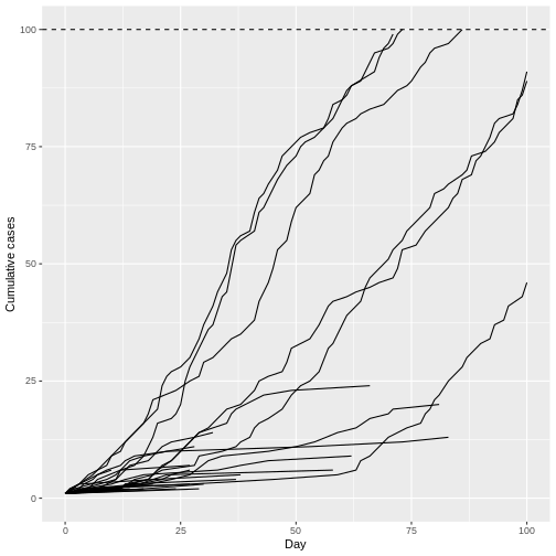
# Visualize transmission chains by cumulative cases
ggplot() +
  # create grouped chain trajectories
  geom_line(
    data = aggregate_chains,
    mapping = aes(
      x = day,
      y = cases_cumsum,
      group = chain
    ),
    color = "black",
    alpha = 0.25,
    show.legend = FALSE
  ) +
  # define a 100-case threshold
  geom_hline(aes(yintercept = 100), lty = 2) +
  labs(
    x = "Day",
    y = "Cumulative cases"
  )
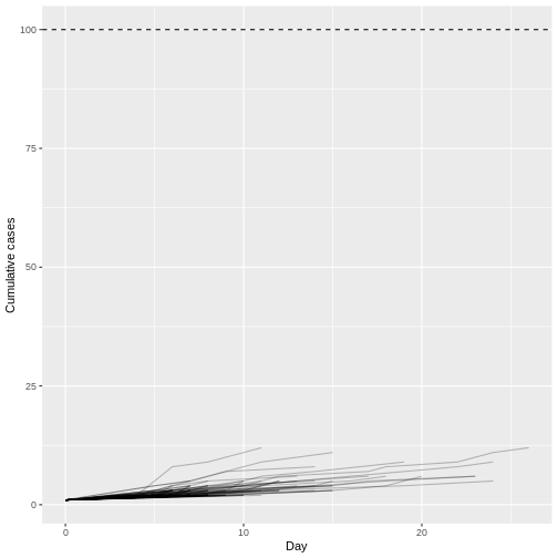
Although most introductions of 1 index case do not generate secondary cases (N = 934) or most outbreaks rapidly become extinct (median duration of 17 and median size of 5.5), only 1 epidemic trajectories among 100 simulations (1%) can reach to more than 100 infected cases. This finding is particularly remarkable because the reproduction number \(R\) is less than 1 (offspring distribution mean of 0.6), but, given an offspring distribution dispersion parameter of 0.02, it shows the potential for explosive outbreaks of MERS disease.
We can count how many chains reached the 100-case threshold using
dplyr functions. This output should give us equivalent
results to summary(multiple_epichains):
R
# number of chains that reached the 100-case threshold
summary_chains %>%
  dplyr::filter(cases_total > 100)
OUTPUT
# A tibble: 1 × 3
  chain day_max cases_total
  <int>   <dbl>       <int>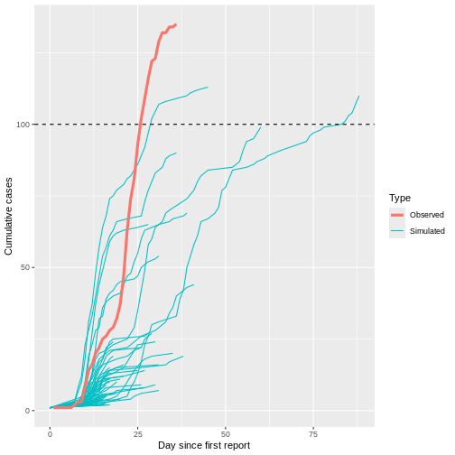
1 65 34 103Let’s overlap the cumulative number of observed cases using the
linelist object from the mers_korea_2015 dataset of the
outbreaks R package. To prepare the dataset so we can
plot daily total cases over time, we use incidence2 to
convert the linelist to an <incidence2> object,
complete the missing dates of the time series with
complete_dates()
R
library(outbreaks)

mers_cumcases <- mers_korea_2015$linelist %>%
  # incidence2 workflow
  incidence2::incidence(date_index = "dt_onset") %>%
  incidence2::complete_dates() %>%
  # wrangling using {dplyr}
  dplyr::mutate(count_cumsum = cumsum(count)) %>%
  tibble::rownames_to_column(var = "day") %>%
  dplyr::mutate(day = as.numeric(day))
Use plot() to make an incidence plot:
R
# plot the incidence2 object
plot(mers_cumcases)
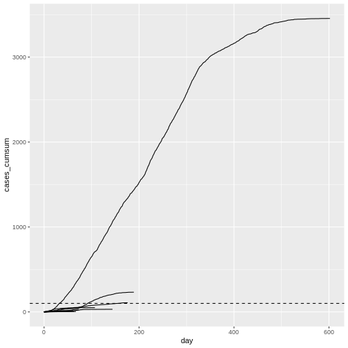
When plotting the observed number of cumulative cases from the Middle East respiratory syndrome (MERS) outbreak in South Korea in 2015 alongside the previously simulated chains, we see that the observed cases followed a trajectory that is consistent with the simulated explosive outbreak dynamics (which makes sense, given the simulation uses parameters based on this specific outbreak).

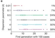
When we increase the dispersion parameter from \(k = 0.01\) to \(k = \infty\) - and hence reduce individual-level variation in transmission - and assume a fixed reproduction number \(R = 1.5\), the proportion of simulated outbreaks that reached the 100-case threshold increases. This is because the simulated outbreaks now have more of a consistent, clockwise dynamic, rather than the high level of variability seen previously.
Early spread projections
In the epidemic’s initial phase, you can use epichains to apply a branching process model to project the number of future cases. Even though the model accounts for randomness in transmission and variation in the number of secondary cases, there may be additional local features we have not considered. Analysis of early forecasts made for COVID in different countries using this model structure found that predictions were often overconfident (Pearson et al., 2020). This is likely because the real-time model did not include all the changes in the offspring distribution that were happening at the local level as a result of behaviour change and control measures. You can read more about the importance of local context in COVID-19 models in Eggo et al. (2020).
We invite you to read the vignette on Projecting infectious disease incidence: a COVID-19 example! for more on making predictions using epichains.
Challenges
Monkeypox large outbreak potential
Evaluate the potential for a new Monkey pox (Mpox) case to generate an explosive large outbreak.
- Simulate 1000 transmission chains with 1 initial case each starting at day 0.
- Use the appropriate package to access delay data from previous outbreaks.
- How many simulated trajectories reach more than 100 infected cases?
With epiparameter, you can access and use offspring and delay distributions from previous Ebola outbreaks.
R
library(epiparameter)
library(tidyverse)

epiparameter::epiparameter_db(epi_name = "offspring") %>%
  epiparameter::parameter_tbl() %>%
  dplyr::count(disease, epi_name)
OUTPUT
# Parameter table:
# A data frame:    6 × 3
  disease                       epi_name                   n
  <chr>                         <chr>                  <int>
1 Ebola Virus Disease           offspring distribution     1
2 Hantavirus Pulmonary Syndrome offspring distribution     1
3 Mpox                          offspring distribution     1
4 Pneumonic Plague              offspring distribution     1
5 SARS                          offspring distribution     2
6 Smallpox                      offspring distribution     4
R
epiparameter::epiparameter_db(epi_name = "serial interval") %>%
  epiparameter::parameter_tbl() %>%
  dplyr::count(disease, epi_name)
OUTPUT
# Parameter table:
# A data frame:    6 × 3
  disease               epi_name            n
  <chr>                 <chr>           <int>
1 COVID-19              serial interval     4
2 Ebola Virus Disease   serial interval     4
3 Influenza             serial interval     1
4 MERS                  serial interval     2
5 Marburg Virus Disease serial interval     2
6 Mpox                  serial interval     5
Also, given that you only need one chain per iteration starting the same day, it may not be necessary to use iteration for this one.
R
# load packages -----------------------------------------------------------

library(epiparameter)
library(tidyverse)

# delays ------------------------------------------------------------------

mpox_offspring_epiparam <- epiparameter::epiparameter_db(
  disease = "mpox",
  epi_name = "offspring",
  single_epiparameter = TRUE
)

mpox_offspring <- epiparameter::get_parameters(mpox_offspring_epiparam)

mpox_serialint <- epiparameter::epiparameter_db(
  disease = "mpox",
  epi_name = "serial interval",
  single_epiparameter = TRUE
)

# iterate -----------------------------------------------------------------

# Set seed for random number generator
set.seed(33)

simulated_chains_mpox <- epichains::simulate_chains(
  n_chains = 1000,
  statistic = "size",
  offspring_dist = rnbinom,
  mu = mpox_offspring["mean"],
  size = mpox_offspring["dispersion"],
  generation_time = function(x) generate(x = mpox_serialint, times = x)
)

# visualize ---------------------------------------------------------------

# daily aggregate of cases
simulated_chains_mpox_day <- simulated_chains_mpox %>%
  # use data.frame output from <epichains> object
  as_tibble() %>%
  # Count the daily number of cases in each chain
  mutate(day = ceiling(time)) %>%
  count(chain, day, name = "cases") %>%
  # Calculate the cumulative number of cases for each chain
  group_by(chain) %>%
  mutate(cumulative_cases = cumsum(cases)) %>%
  ungroup()

# Visualize transmission chains by cumulative cases
simulated_chains_mpox_day %>%
  # Create grouped chain trajectories
  ggplot(aes(x = day, y = cumulative_cases, group = chain)) +
  geom_line(color = "black", alpha = 0.25, show.legend = FALSE) +
  # Define a 100-case threshold
  geom_hline(aes(yintercept = 100), lty = 2) +
  labs(x = "Day", y = "Cumulative cases")
Assuming a Monkey pox outbreak with \(R\) = 0.32 and \(k\) = 0.58, there is no trajectory among 1000 simulations that reach more than 100 infected cases. Compared to MERS (\(R\) = 0.6 and \(k\) = 0.02).
With superspreading, you can get numerical solutions to processes that epichains solve using branching processes. We invite you to read the superspreading vignette on Epidemic risk and respond to:
- What is the probability that a newly introduced pathogen will cause a large outbreak?
- What is the probability that an infection will, by chance, fail to establish following initial introduction(s)?
- What is the probability the outbreak will be contained?
Check how these estimates vary non-linearly with respect to the mean reproduction number \(R\) and dispersion \(k\) of a given disease.
From a distribution of secondary cases
Christian Althaus, 2015 reused data published by Faye et al., 2015 (Figure 2) on the transmission tree on Ebola virus disease in Conakry, Guinea, 2014.
Using the data under the hint tab:
- Estimate the offspring distribution from the distribution of secondary cases.
- Then estimate the large outbreak potential from this data, simulating 100 runs with one initial case.
- Print the summary of the
<epichains>class object. This should help us count how many chains reach asizeof more than 100 infected cases.
For reproducible results use set.seed(645).
Code with the transmission tree data written by Christian Althaus, 2015:
R
# Number of individuals in the trees
n <- 152
# Number of secondary cases for all individuals
c1 <- c(1, 2, 2, 5, 14, 1, 4, 4, 1, 3, 3, 8, 2, 1, 1,
4, 9, 9, 1, 1, 17, 2, 1, 1, 1, 4, 3, 3, 4, 2,
5, 1, 2, 2, 1, 9, 1, 3, 1, 2, 1, 1, 2)
c0 <- c(c1, rep(0, n - length(c1)))
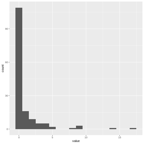
c0 %>%
enframe() %>%
ggplot(aes(value)) +
geom_histogram(binwidth = 1)
Optional challenge:
- Reproduce Figure (B) from Christian Althaus, 2015 with the simulation output.
R
# load packages ---------------------------
library(epichains)
library(epiparameter)
library(fitdistrplus)
library(tidyverse)
R
# fit a negative binomial distribution ------------------------------------

# Fitting a negative binomial distribution to the number of secondary cases
fit.cases <- fitdistrplus::fitdist(c0, "nbinom")
fit.cases
OUTPUT
Fitting of the distribution ' nbinom ' by maximum likelihood
Parameters:
      estimate Std. Error
size 0.1814260 0.03990278
mu   0.9537995 0.19812301
R
# serial interval parameters ----------------------------------------------

ebola_serialinter <- epiparameter::epiparameter_db(
  disease = "ebola",
  epi_name = "serial interval",
  single_epiparameter = TRUE
)

# simulate outbreak trajectories ------------------------------------------

# Set seed for random number generator
set.seed(645)
sim_multiple_chains <- epichains::simulate_chains(
  n_chains = 100,
  statistic = "size",
  offspring_dist = rnbinom,
  mu = fit.cases$estimate["mu"],
  size = fit.cases$estimate["size"],
  generation_time = function(x) generate(x = ebola_serialinter, times = x)
)

# summarise ----------------------------------------

summary(sim_multiple_chains)
OUTPUT
`epichains_summary` object

  [1]    9    1    2    1    1    4    1   20   14    1    1  131    1    2    1
 [16]    1    7    1    2 2889    1    1    1   13    3    1    1    1    1    1
 [31]    5    6    1    1    1    1    1    1    1    1    2    1    1    2    1
 [46]    1    1    1    1    1    1    1    1    1  335    1   11    3   24    6
 [61]    1    1    1    1    1    1    1    1    1    1    1    1    1    1  111
 [76]    1    1    1    1    1    1    2    1  544    1    1    1    3    1    2
 [91]    6    1    1    1    1    1    1    1 2091    1

 Simulated sizes:

Max: 2889
Min: 1
R
# visualize ----------------------------------------
sim_chains_aggregate <-
sim_multiple_chains %>%
# use data.frame output from <epichains> object
as_tibble() %>%
# Count the daily number of cases in each chain
mutate(day = ceiling(time)) %>%
count(chain, day, name = "cases") %>%
# Calculate the cumulative number of cases for each chain
group_by(chain) %>%
mutate(cumulative_cases = cumsum(cases)) %>%
ungroup()
sim_chains_aggregate %>%
# Create grouped chain trajectories
ggplot(aes(x = day, y = cumulative_cases, group = chain)) +
geom_line() +
# Define a 100-case threshold
geom_hline(aes(yintercept = 100), lty = 2) +
ylim(0, 100) +
xlim(0, 100) +
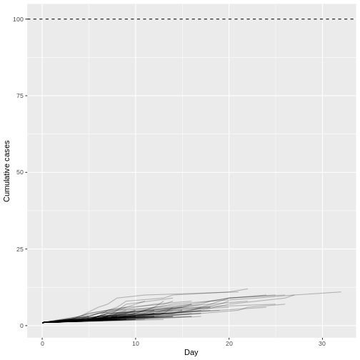
labs(x = "Day", y = "Cumulative cases")
Remarkably, even with R0 less than 1 (R = 0.95) we can have potentially explosive outbreaks. The observed variation in individual infectiousness in Ebola means that although the probability of extinction is high, new index cases also have the potential for explosive regrowth of the epidemic.
- Use epichains to simulate the large outbreak potential of diseases with overdispersed offspring distributions.