Create a short-term forecast
Last updated on 2026-07-01 | Edit this page
Estimated time: 60 minutes
Overview
Questions
- How do I create short-term forecasts from case data?
- How do I account for incomplete reporting in forecasts?
Objectives
- Learn how to make forecasts of cases using R package
EpiNow2 - Learn how to include an observation process in estimation
Prerequisites
- Complete tutorial Quantifying transmission
Learners should familiarise themselves with following concept dependencies before working through this tutorial:
Statistics: probability distributions, principle of Bayesian analysis.
Epidemic theory: Effective reproduction number.
Introduction
Given case data of an epidemic, we can create estimates of the current and future number of cases by accounting for both delays in reporting and under reporting. To make predictions about the future course of the epidemic, we need to make an assumption of how observations up to the present are related to what we expect to happen in the future. The simplest way of doing so is to assume “no change”, i.e., the reproduction number remains the same in the future as last observed. In this tutorial we will create short-term forecasts by assuming the reproduction number will remain the same as its estimate was on the final date for which data was available.
In this tutorial we are going to learn how to use the EpiNow2 package to forecast cases accounting for incomplete observations and forecast secondary observations like deaths.
We’ll use the pipe %>% operator to connect functions,
so let’s also call to the tidyverse package:
R
library(EpiNow2)
library(tidyverse)
The double-colon
The double-colon :: in R let you call a specific
function from a package without loading the entire package into the
current environment.
For example, dplyr::filter(data, condition) uses
filter() from the dplyr package.
This helps us remember package functions and avoid namespace conflicts.
Create a short-term forecast
The function epinow() described in the quantifying transmission
episode is a wrapper for the functions:
-
estimate_infections()used to estimate cases by date of infection. -
forecast_infections()used to simulate infections using an existing fit (estimate) to observed cases.
Let’s use the same code used in quantifying transmission episode to get the input data, delays and priors:
R
# Read cases dataset
cases <- incidence2::covidregionaldataUK %>%
  # use {tidyr} to preprocess missing values
  tidyr::replace_na(base::list(cases_new = 0)) %>%
  # use {incidence2} to compute the daily incidence
  incidence2::incidence(
    date_index = "date",
    counts = "cases_new",
    count_values_to = "confirm",
    date_names_to = "date",
    complete_dates = TRUE
  ) %>%
  dplyr::select(-count_variable)  # Drop count_variable as no longer needed

# Incubation period
incubation_period_fixed <- EpiNow2::Gamma(
  mean = 4,
  sd = 2,
  max = 20
)

# Log-tranformed mean
log_mean <- EpiNow2::convert_to_logmean(mean = 2, sd = 1)

# Log-transformed std
log_sd <- EpiNow2::convert_to_logsd(mean = 2, sd = 1)

# Reporting delay
reporting_delay_fixed <- EpiNow2::LogNormal(
  mean = log_mean,
  sd = log_sd,
  max = 10
)

# Generation time
generation_time_fixed <- EpiNow2::LogNormal(
  mean = 3.6,
  sd = 3.1,
  max = 20
)

# define Rt prior distribution
rt_prior <- EpiNow2::rt_opts(prior = EpiNow2::LogNormal(mean = 2, sd = 2))
Now we can extract the short-term forecast using:
R
# Assume we only have the first 90 days of this data
reported_cases <- cases %>%
  dplyr::slice(1:90)

# Estimate and forecast
estimates <- EpiNow2::epinow(
  data = reported_cases,
  generation_time = EpiNow2::generation_time_opts(generation_time_fixed),
  delays = EpiNow2::delay_opts(incubation_period_fixed + reporting_delay_fixed),
  rt = rt_prior
)
Do not wait for this to complete!
This last chunk may take 10 minutes to run. Keep reading this tutorial episode while this runs in the background. For more information on computing time, read the “Bayesian inference using Stan” section within the quantifying transmission episode.
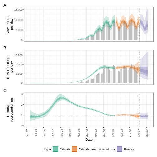
We can visualise the estimates of the effective reproduction number
and the estimated number of cases using plot(). The
estimates are split into three categories:
Estimate (green): utilises all data,
Estimate based on partial data (orange): contains a higher degree of uncertainty because such estimates are based on less data,
Forecast (purple): forecasts into the future.
R
plot(estimates)
Forecasting with incomplete observations
In the quantifying
transmission episode we accounted for delays in reporting. In
EpiNow2 we also can account for incomplete observations as
in reality, 100% of cases are not reported. We will pass an additional
argument called obs into the epinow() function
to define an observation model. The format of obs is
defined by the obs_opt() function (see
?EpiNow2::obs_opts for more detail).
Let’s say we believe the COVID-19 outbreak data in the
cases object do not include all reported cases. We estimate
that only 40% of actual cases are reported. To specify this in the
observation model, we must pass a scaling factor with a mean and
standard deviation. If we assume that 40% of cases are reported (with
standard deviation 1%), then we specify the scale input to
obs_opts() as follows:
R
obs_scale <- EpiNow2::Normal(mean = 0.4, sd = 0.01)
To run the inference framework with this observation process, we add
obs = obs_opts(scale = obs_scale) to the input arguments of
epinow():
R
# Define observation model
obs_scale <- EpiNow2::Normal(mean = 0.4, sd = 0.01)

# Assume we only have the first 90 days of this data
reported_cases <- cases %>%
  dplyr::slice(1:90)

# Estimate and forecast
estimates <- EpiNow2::epinow(
  data = reported_cases,
  generation_time = EpiNow2::generation_time_opts(generation_time_fixed),
  delays = EpiNow2::delay_opts(incubation_period_fixed + reporting_delay_fixed),
  rt = rt_prior,
  # Add observation model
  obs = EpiNow2::obs_opts(scale = obs_scale)
)

base::summary(estimates)
OUTPUT
                        measure                 estimate
                         <char>                   <char>
1:       New infections per day   20133 (13352 -- 29484)
2:   Expected change in reports        Likely decreasing
3:   Effective reproduction no.       0.97 (0.77 -- 1.2)
4:               Rate of growth -0.012 (-0.092 -- 0.066)
5: Doubling/halving time (days)         -58 (10 -- -7.5)
The estimates of transmission measures such as the effective reproduction number and rate of growth are similar (or the same in value) compared to when we didn’t account for incomplete observations (see quantifying transmission episode in the “Finding estimates” section). However the number of new confirmed cases by infection date has changed substantially in magnitude to reflect the assumption that only 40% of cases are reported.
We can also change the default distribution from Negative Binomial to
Poisson, remove the default week effect (which accounts for weekly
patterns in reporting) and more. See ?EpiNow2::obs_opts for
more details.
What are the implications of this change?
- Compare different percents of observations %
- How are they different in the number of infections estimated?
- What are the public health implications of this change?
Forecasting secondary observations
EpiNow2 also has the ability to estimate and forecast
secondary observations, e.g., deaths and hospitalisations, from a
primary observation, e.g., cases. Here we will illustrate how to
forecast the number of deaths arising from observed cases of COVID-19 in
the early stages of the UK outbreak.
First, we must format our data to have the following columns:
-
date: the date (as a date object see?is.Date()), -
primary: number of primary observations on that date, in this example cases, -
secondary: number of secondary observations date, in this example deaths.
R
reported_cases_deaths <- incidence2::covidregionaldataUK %>%
  # use {tidyr} to preprocess missing values
  tidyr::replace_na(base::list(cases_new = 0, deaths_new = 0)) %>%
  # use {incidence2} to compute the daily incidence
  incidence2::incidence(
    date_index = "date",
    counts = c(primary = "cases_new", secondary = "deaths_new"),
    date_names_to = "date",
    complete_dates = TRUE
  ) %>%
  # rearrange to wide format for {EpiNow2}
  pivot_wider(names_from = count_variable, values_from = count)
Using the data on cases and deaths between day 31 and day 60, we will
estimate the relationship between the primary and secondary observations
using estimate_secondary(), then forecast future deaths
using forecast_secondary(). For more details on the model
see the model
documentation.
We must specify the type of observation using type in
secondary_opts(), options include:
- “incidence”: secondary observations arise from previous primary observations, i.e., deaths arising from recorded cases.
- “prevalence”: secondary observations arise from a combination current primary observations and past secondary observations, i.e., hospital bed usage arising from current hospital admissions and past hospital bed usage.
In this example we specify
secondary_opts(type = "incidence"). See
?EpiNow2::secondary_opts for more detail.
The final key input is the delay distribution between the primary and
secondary observations. Here this is the delay between case report and
death, we assume this follows a gamma distribution with mean of 14 days
and standard deviation of 5 days (Alternatively, we can use
epiparameter to access
epidemiological delays). Using Gamma() we specify a
fixed gamma distribution.
There are further function inputs to
estimate_secondary() which can be specified, including
adding an observation process, see
?EpiNow2::estimate_secondary for detail on these
options.
To find the model fit between cases and deaths:
R
# Estimate from day 31 to day 60 of this data
cases_to_estimate <- reported_cases_deaths %>%
  slice(31:60)

# Delay distribution between case report and deaths
delay_report_to_death <- EpiNow2::Gamma(
  mean = EpiNow2::Normal(mean = 14, sd = 0.5),
  sd = EpiNow2::Normal(mean = 5, sd = 0.5),
  max = 30
)

# Estimate secondary cases
estimate_cases_to_deaths <- EpiNow2::estimate_secondary(
  data = cases_to_estimate,
  secondary = EpiNow2::secondary_opts(type = "incidence"),
  delays = EpiNow2::delay_opts(delay_report_to_death)
)
Be cautious of time-scale
In the early stages of an outbreak there can be substantial changes in testing and reporting. If there are testing changes from one month to another, then there will be a bias in the model fit. Therefore, you should be cautious of the time-scale of data used in the model fit and forecast.
We plot the model fit (shaded ribbons) with the secondary observations (bar plot) and primary observations (dotted line) as follows:
R
plot(estimate_cases_to_deaths, primary = TRUE)
WARNING
Warning: Removed 14 rows containing missing values or values outside the scale range
(`geom_ribbon()`).
Removed 14 rows containing missing values or values outside the scale range
(`geom_ribbon()`).
Removed 14 rows containing missing values or values outside the scale range
(`geom_ribbon()`).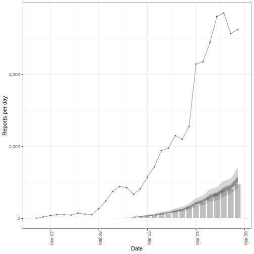
To use this model fit to forecast deaths, we pass a data frame consisting of the primary observation (cases) for dates not used in the model fit.
Note : in this episode we are using data where we know the deaths and cases, so we create a data frame by extracting the cases. But in practice, this would be a different data set consisting of cases only.
R
# Forecast from day 61 to day 90
cases_to_forecast <- reported_cases_deaths %>%
  dplyr::slice(61:90) %>%
  dplyr::mutate(value = primary)
To forecast, we use the model fit
estimate_cases_to_deaths:
R
# Forecast secondary cases
deaths_forecast <- EpiNow2::forecast_secondary(
  estimate = estimate_cases_to_deaths,
  primary = cases_to_forecast
)

plot(deaths_forecast)
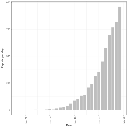
The plot shows the forecast secondary observations (deaths) over the
dates which we have recorded cases for. It is also possible to forecast
deaths using forecast cases, here you would specify primary
as the estimates output from
estimate_infections().
Credible intervals
In all EpiNow2 output figures, shaded regions reflect 90%, 50%, and 20% credible intervals in order from lightest to darkest.
Challenge: Ebola outbreak analysis
Challenge
Download the file ebola_cases.csv and read it
into R. The simulated data consists of the date of symptom onset and
number of confirmed cases of the early stages of the Ebola outbreak in
Sierra Leone in 2014.
Using the first 3 months (120 days) of data:
- Estimate whether cases are increasing or decreasing on day 120 of the outbreak
- Account for a capacity to observe 80% of cases.
- Create a two week forecast of number of cases.
You can use the following parameter values for the delay distribution(s) and generation time distribution.
- Incubation period: Log normal\((2.487,0.330)\) (Eichner et al. 2011 via epiparameter)
- Generation time: Gamma\((15.3, 10.1)\) (WHO Ebola Response Team 2014)
You may include some uncertainty around the mean and standard deviation of these distributions.
We use the effective reproduction number and growth rate to estimate whether cases are increasing or decreasing.
We can use the horizon argument within the
forecast_opts() provided to forecast argument
in epinow() function to extend the time period of the
forecast. The default value is of seven days.
Ensure the data is in the correct format :
-
date: the date (as a date object see?is.Date()), -
confirm: number of confirmed cases on that date.
To estimate the effective reproduction number and growth rate, we
will use the function epinow().
As the data consists of date of symptom onset, we only need to specify a delay distribution for the incubation period and the generation time.
We specify the distributions with some uncertainty around the mean and standard deviation of the log normal distribution for the incubation period and the Gamma distribution for the generation time.
R
epiparameter::epiparameter_db(
  disease = "ebola",
  epi_name = "incubation"
) %>%
  epiparameter::parameter_tbl()
OUTPUT
# Parameter table:
# A data frame:    5 × 7
  disease           pathogen epi_name prob_distribution author  year sample_size
  <chr>             <chr>    <chr>    <chr>             <chr>  <dbl>       <dbl>
1 Ebola Virus Dise… Ebola V… incubat… lnorm             Eichn…  2011         196
2 Ebola Virus Dise… Ebola V… incubat… gamma             WHO E…  2015        1798
3 Ebola Virus Dise… Ebola V… incubat… gamma             WHO E…  2015          49
4 Ebola Virus Dise… Ebola V… incubat… gamma             WHO E…  2015         957
5 Ebola Virus Dise… Ebola V… incubat… gamma             WHO E…  2015         792
R
ebola_eichner <- epiparameter::epiparameter_db(
  disease = "ebola",
  epi_name = "incubation",
  author = "Eichner"
)

ebola_eichner_parameters <- epiparameter::get_parameters(ebola_eichner)

ebola_incubation_period <- EpiNow2::LogNormal(
  meanlog = EpiNow2::Normal(
    mean = ebola_eichner_parameters["meanlog"],
    sd = 0.5
  ),
  sdlog = EpiNow2::Normal(
    mean = ebola_eichner_parameters["sdlog"],
    sd = 0.5
  ),
  max = 20
)

ebola_generation_time <- EpiNow2::Gamma(
  mean = EpiNow2::Normal(mean = 15.3, sd = 0.5),
  sd = EpiNow2::Normal(mean = 10.1, sd = 0.5),
  max = 30
)
We read the data input using readr::read_csv(). This
function recognize that the column date is a
<date> class vector.
R
# read data
# e.g.: if path to file is data/raw-data/ebola_cases.csv then:
ebola_cases_raw <- readr::read_csv(
  here::here("data", "raw-data", "ebola_cases.csv")
)
Preprocess and adapt the raw data for EpiNow2:
R
ebola_cases <- ebola_cases_raw %>%
  # use {tidyr} to preprocess missing values
  tidyr::replace_na(base::list(confirm = 0)) %>%
  # use {incidence2} to compute the daily incidence
  incidence2::incidence(
    date_index = "date",
    counts = "confirm",
    count_values_to = "confirm",
    date_names_to = "date",
    complete_dates = TRUE
  ) %>%
  dplyr::select(-count_variable)

dplyr::as_tibble(ebola_cases)
OUTPUT
# A tibble: 123 × 2
   date       confirm
   <date>       <dbl>
 1 2014-05-18       1
 2 2014-05-19       0
 3 2014-05-20       2
 4 2014-05-21       4
 5 2014-05-22       6
 6 2014-05-23       1
 7 2014-05-24       2
 8 2014-05-25       0
 9 2014-05-26      10
10 2014-05-27       8
# ℹ 113 more rows
We define an observation model to scale the estimated and forecast number of new infections:
R
# Define observation model
# mean of 80% and standard deviation of 1%
ebola_obs_scale <- EpiNow2::Normal(mean = 0.8, sd = 0.01)
As we want to also create a two week forecast, we specify
horizon = 14 to forecast 14 days instead of the default 7
days.
R
ebola_estimates <- EpiNow2::epinow(
  data = ebola_cases %>% dplyr::slice(1:120), # first 3 months of data only
  generation_time = EpiNow2::generation_time_opts(ebola_generation_time),
  delays = EpiNow2::delay_opts(ebola_incubation_period),
  # Add observation model
  obs = EpiNow2::obs_opts(scale = ebola_obs_scale),
  # horizon needs to be 14 days to create two week forecast (default is 7 days)
  forecast = EpiNow2::forecast_opts(horizon = 14)
)

summary(ebola_estimates)
OUTPUT
                        measure                estimate
                         <char>                  <char>
1:       New infections per day          91 (50 -- 186)
2:   Expected change in reports              Increasing
3:   Effective reproduction no.        1.6 (1.2 -- 2.4)
4:               Rate of growth 0.041 (0.0029 -- 0.087)
5: Doubling/halving time (days)         17 (7.9 -- 240)
The effective reproduction number \(R_t\) estimate (on the last date of the data) is 1.6 (1.2 – 2.4). The exponential growth rate of case numbers is 0.041 (0.0029 – 0.087).
Visualize the estimates:
R
plot(ebola_estimates)
Forecasting with estimates of \(R_t\)
By default, the short-term forecasts are created using the latest estimate of the reproduction number \(R_t\). As this estimate is based on partial data, it has considerable uncertainty.
The reproduction number that is projected into the future can be
changed to a less recent estimate based on more data using
rt_opts():
R
EpiNow2::rt_opts(future = "estimate")
The result will be less uncertain forecasts (as they are based on \(R_t\) with a narrower uncertainty interval) but the forecasts will be based on less recent estimates of \(R_t\) and assume no change since then.
Additionally, there is the option to project the value of \(R_t\) into the future using a generic model
by setting future = "project". As this option uses a model
to forecast the value of \(R_t\), the
result will be forecasts that are more uncertain than
estimate, for an example see
here.
Summary
EpiNow2 can be used to create short term forecasts and
to estimate the relationship between different outcomes. There are a
range of model options that can be implemented for different analysis,
including adding an observational process to account for incomplete
reporting. See the vignette
for more details on different model options in EpiNow2 that
aren’t covered in these tutorials.
- We can create short-term forecasts by making assumptions about the future behaviour of the reproduction number
- Incomplete case reporting can be accounted for in estimates