Quantifying transmission

Last updated on 2025-10-17 | Edit this page

Estimated time: 30 minutes

Overview

Questions

How can I estimate the time-varying reproduction number ($Rt$) and growth rate from a time series of case data?
How can I quantify geographical heterogeneity from these transmission metrics?

Objectives

Learn how to estimate transmission metrics from a time series of case data using the R package EpiNow2

Prerequisites

Learners should familiarise themselves with following concepts before working through this tutorial:

Statistics: probability distributions, principle of Bayesian analysis.

Epidemic theory: Effective reproduction number.

Data science: Data transformation and visualization. You can review the episode on Aggregate and visualize incidence data.

Reminder: the Effective Reproduction Number, $R_t$

The basic reproduction number, $R_0$, is the average number of cases caused by one infectious individual in an entirely susceptible population.

But in an ongoing outbreak, the population does not remain entirely susceptible as those that recover from infection are typically immune. Moreover, there can be changes in behaviour or other factors that affect transmission. When we are interested in monitoring changes in transmission we are therefore more interested in the value of the effective reproduction number, $R_t$, which represents the average number of cases caused by one infectious individual in the population at time $t$, given the current state of the population (including immunity levels and control measures).

Introduction

The transmission intensity of an outbreak is quantified using two key metrics: the reproduction number, which informs on the strength of the transmission by indicating how many new cases are expected from each existing case; and the growth rate, which informs on the speed of the transmission by indicating how rapidly the outbreak is spreading or declining (doubling/halving time) within a population. For more details on the distinction between speed and strength of transmission and implications for control, review Dushoff & Park, 2021.

To estimate these key metrics using case data we must account for delays between the date of infections and date of reported cases. In an outbreak situation, data are usually available on reported dates only, therefore we must use estimation methods to account for these delays when trying to understand changes in transmission over time.

In the next tutorials we will focus on how to use the functions in EpiNow2 to estimate transmission metrics of case data. We will not cover the theoretical background of the models or inference framework, for details on these concepts see the vignette.

In this tutorial we are going to learn how to use the EpiNow2 package to estimate the time-varying reproduction number. We’ll get input data from incidence2. We’ll use the tidyr and dplyr packages to arrange some of its outputs, ggplot2 to visualize case distribution, and the pipe %>% to connect some of their functions, so let’s also call to the tidyverse package:

R

library(EpiNow2)
library(incidence2)
library(tidyverse)

The double-colon

The double-colon :: in R lets you call a specific function from a package without loading the entire package into the current environment.

For example, dplyr::filter(data, condition) uses filter() from the dplyr package.

This helps us remember package functions and avoid namespace conflicts.

Instructor Note

This tutorial illustrates the usage of epinow() to estimate the time-varying reproduction number and infection times. Learners should understand the necessary inputs to the model and the limitations of the model output.

Bayesian inference

The R package EpiNow2 uses a Bayesian inference framework to estimate reproduction numbers and infection times based on reporting dates. In other words, it estimates transmission based on when people were actually infected (rather than symptom onset), by accounting for delays in observed data. In contrast, the EpiEstim package allows faster and simpler real-time estimation of the reproduction number using only case data over time, reflecting how transmission changes based on when symptoms appear.

In Bayesian inference, we use prior knowledge (prior distributions) with data (in a likelihood function) to find the posterior probability:

$Posterior \, probability \propto likelihood \times prior \, probability$

Instructor Note

Refer to the prior probability distribution and the posterior probability distribution.

In the “Expected change in reports” callout, by “the posterior probability that $R_t < 1$”, we refer specifically to the area under the posterior probability distribution curve.

Delay distributions and case data

Case data

To illustrate the functions of EpiNow2 we will use outbreak data of the start of the COVID-19 pandemic from the United Kingdom, but only with the first 90 days observed. The data are available in the R package incidence2.

R

dplyr::as_tibble(incidence2::covidregionaldataUK)

OUTPUT

# A tibble: 6,370 × 13
   date       region   region_code cases_new cases_total deaths_new deaths_total
   <date>     <chr>    <chr>           <dbl>       <dbl>      <dbl>        <dbl>
 1 2020-01-30 East Mi… E12000004          NA          NA         NA           NA
 2 2020-01-30 East of… E12000006          NA          NA         NA           NA
 3 2020-01-30 England  E92000001           2           2         NA           NA
 4 2020-01-30 London   E12000007          NA          NA         NA           NA
 5 2020-01-30 North E… E12000001          NA          NA         NA           NA
 6 2020-01-30 North W… E12000002          NA          NA         NA           NA
 7 2020-01-30 Norther… N92000002          NA          NA         NA           NA
 8 2020-01-30 Scotland S92000003          NA          NA         NA           NA
 9 2020-01-30 South E… E12000008          NA          NA         NA           NA
10 2020-01-30 South W… E12000009          NA          NA         NA           NA
# ℹ 6,360 more rows
# ℹ 6 more variables: recovered_new <dbl>, recovered_total <dbl>,
#   hosp_new <dbl>, hosp_total <dbl>, tested_new <dbl>, tested_total <dbl>

To use the data, we must format the data to have two columns:

date: the date (as a date object see ?is.Date()),
confirm: number of disease reports (confirm) on that date.

Let’s use tidyr and incidence2 for this:

R

cases_sliced <- incidence2::covidregionaldataUK %>%
  tibble::as_tibble() %>%
  # Preprocess missing values
  tidyr::replace_na(base::list(cases_new = 0)) %>%
  # Compute the daily incidence
  incidence2::incidence(
    date_index = "date",
    counts = "cases_new",
    count_values_to = "confirm",
    date_names_to = "date",
    complete_dates = TRUE
  ) %>%
  # Keep the first 90 dates
  dplyr::slice_head(n = 90)

With incidence2::incidence() we aggregate cases in different time intervals (i.e., days, weeks or months) or per group categories. Also we can have complete dates for all the range of dates per group category using complete_dates = TRUE Explore later the incidence2::incidence() reference manual

Show details

Can we replicate {incidence2} with {dplyr}?

We can get an object similar to cases from the incidence2::covidregionaldataUK data frame using the dplyr package.

R

incidence2::covidregionaldataUK %>%
  dplyr::select(date, cases_new) %>%
  dplyr::group_by(date) %>%
  dplyr::summarise(confirm = sum(cases_new, na.rm = TRUE)) %>%
  dplyr::ungroup() %>%
  dplyr::slice_head(n = 90)

However, the incidence2::incidence() function contains convenient arguments like complete_dates that facilitate getting an incidence object with the same range of dates for each grouping without the need of extra code lines or a time-series package.

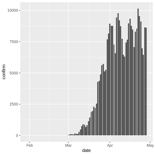
In an outbreak situation it is likely we would only have access to the beginning of the input data set. Therefore we assume we only have the first 90 days of this data.

R

plot(cases_sliced)

To pass the outputs from incidence2 to EpiNow2 we need to drop one column from the cases_sliced object:

R

# Drop column for {EpiNow2} input format
cases <- cases_sliced %>%
  dplyr::select(-count_variable)

cases

OUTPUT

# A tibble: 90 × 2
   date       confirm
   <date>       <dbl>
 1 2020-01-30       3
 2 2020-01-31       0
 3 2020-02-01       0
 4 2020-02-02       0
 5 2020-02-03       0
 6 2020-02-04       0
 7 2020-02-05       2
 8 2020-02-06       0
 9 2020-02-07       0
10 2020-02-08       8
# ℹ 80 more rows

Delay distributions

We assume there are delays from the time of infection until the time a case is reported. We specify these delays as distributions to account for the uncertainty in individual level differences. The delay may involve multiple types of processes. A typical delay from time of infection to case reporting may consist of:

time from infection to symptom onset (the incubation period) + time from symptom onset to case notification (the reporting time) .

The delay distribution for each of these processes can either estimated from data or obtained from the literature. We can express uncertainty about what the correct parameters of the distributions by assuming the distributions have fixed parameters or whether they have variable parameters. To understand the difference between fixed and variable distributions, let’s consider the incubation period.

Delays and data

The number of delays and type of delay are a flexible input that depend on the data. The examples below highlight how the delays can be specified for different data sources:

Data source	Delay(s)
Time of symptom onset	Incubation period
Time of case report	Incubation period + time from symptom onset to case notification
Time of hospitalisation	Incubation period + time from symptom onset to hospitalisation

Incubation period distribution

The distribution of incubation period for many diseases can usually be obtained from the literature. The package epiparameter contains a library of epidemiological parameters for different diseases obtained from the literature.

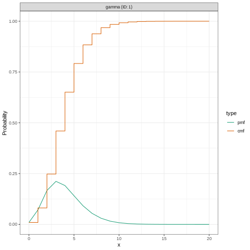
We specify a (fixed) gamma distribution with mean $\mu = 4$ and standard deviation $\sigma = 2$ (shape = $4$, scale = $1$) using the function Gamma() as follows:

R

incubation_period_fixed <- EpiNow2::Gamma(
  mean = 4,
  sd = 2,
  max = 20
)

incubation_period_fixed

OUTPUT

- gamma distribution (max: 20):
  shape:
    4
  rate:
    1

The argument max is the maximum value the distribution can take; in this example, 20 days.

We can plot distributions generated by EpiNow2 using plot():

R

plot(incubation_period_fixed)

Why a gamma distribution?

The incubation period must be a positive value. Therefore we must specify a distribution in EpiNow2 which is for positive values only.

Gamma() supports Gamma distributions and LogNormal() Log-normal distributions, which are distributions for positive values only.

For all types of delay, we will need to use distributions for positive values only - we don’t want to include delays of negative days in our analysis!

Including distribution uncertainty

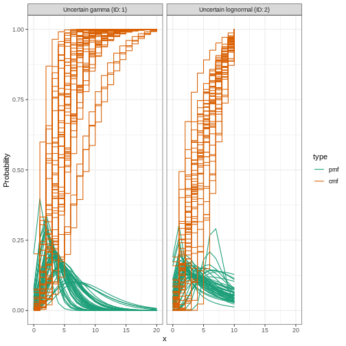
To specify a variable distribution, we include uncertainty around the mean $\mu$ and standard deviation $\sigma$ of our gamma distribution. If our incubation period distribution has a mean $\mu$ and standard deviation $\sigma$, then we assume the mean ($\mu$) follows a Normal distribution with standard deviation $\sigma_{\mu}$:

\[\mbox{Normal}(\mu,\sigma_{\mu}^2)\]

and a standard deviation ($\sigma$) follows a Normal distribution with standard deviation $\sigma_{\sigma}$:

\[\mbox{Normal}(\sigma,\sigma_{\sigma}^2).\]

We specify this using Normal() for each argument: the mean ($\mu = 4$ with $\sigma_{\mu} = 0.5$) and standard deviation ($\sigma = 2$ with $\sigma_{\sigma} = 0.5$).

R

incubation_period_variable <- EpiNow2::Gamma(
  mean = EpiNow2::Normal(mean = 4, sd = 0.5),
  sd = EpiNow2::Normal(mean = 2, sd = 0.5),
  max = 20
)

incubation_period_variable

OUTPUT

- gamma distribution (max: 20):
  shape:
    - normal distribution:
      mean:
        4
      sd:
        0.61
  rate:
    - normal distribution:
      mean:
        1
      sd:
        0.31

Let’s plot the distribution we just configured:

R

plot(incubation_period_variable)

Reporting delays

After the incubation period, there will be an additional delay of time from symptom onset to case notification: the reporting delay. We can specify this as a fixed or variable distribution, or estimate a distribution from data.

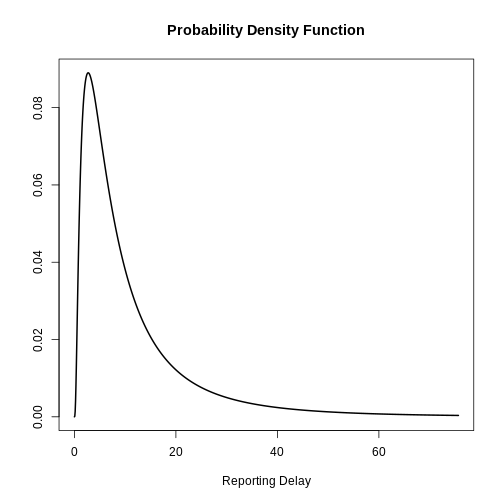
When specifying a distribution, it is useful to visualise the probability density to see the peak and spread of the distribution, in this case we will use a log normal distribution.

If we want to assume that the mean reporting delay is 2 days (with a uncertainty of 0.5 days) and a standard deviation of 1 day (with uncertainty of 0.5 days), we can specify a variable distribution using LogNormal() as before:

R

reporting_delay_variable <- EpiNow2::LogNormal(
  meanlog = EpiNow2::Normal(mean = 2, sd = 0.5),
  sdlog = EpiNow2::Normal(mean = 1, sd = 0.5),
  max = 10
)

Show details

Visualize a log Normal distribution using {epiparameter}

Using epiparameter::epiparameter() we can create a custom distribution. The fixed log normal distribution will look like:

R

library(epiparameter)

R

epiparameter::epiparameter(
  disease = "covid",
  epi_name = "reporting delay",
  prob_distribution =
    epiparameter::create_prob_distribution(
      prob_distribution = "lnorm",
      prob_distribution_params = c(
        meanlog = 2,
        sdlog = 1
      )
    )
) %>%
  plot()

Show details

How to get the reporting delay from data?

If data is available on the time between symptom onset and reporting, we can use the function EpiNow2::estimate_delay() to estimate a log normal distribution from a vector of delays.

The code below illustrates how to use EpiNow2::estimate_delay() with synthetic Ebola data. We calculate the reporting delay for each case the time difference from date of onset to date of hospitalization (date when case was reported).

R

library(tidyverse)

# Steps:
# - get Ebola data from package {outbreaks}
# - keep a subset of columns for this example only
# - calculate the time difference between two dates in linelist
# - extract the time difference as a vector class object
# - estimate the delay parameters using {EpiNow2}

outbreaks::ebola_sim_clean$linelist %>%
  tibble::as_tibble() %>%
  dplyr::select(case_id, date_of_onset, date_of_hospitalisation) %>%
  dplyr::mutate(reporting_delay = date_of_hospitalisation - date_of_onset) %>%
  dplyr::pull(reporting_delay) %>%
  EpiNow2::estimate_delay(
    samples = 1000,
    bootstraps = 10
  )

OUTPUT

WARN [2025-10-17 15:54:35] dist_fit (chain: 1): The largest R-hat is 1.1, indicating chains have not mixed.
Running the chains for more iterations may help. See
https://mc-stan.org/misc/warnings.html#r-hat -
WARN [2025-10-17 15:54:35] dist_fit (chain: 1): Bulk Effective Samples Size (ESS) is too low, indicating posterior means and medians may be unreliable.
Running the chains for more iterations may help. See
https://mc-stan.org/misc/warnings.html#bulk-ess -
WARN [2025-10-17 15:54:35] dist_fit (chain: 1): Tail Effective Samples Size (ESS) is too low, indicating posterior variances and tail quantiles may be unreliable.
Running the chains for more iterations may help. See
https://mc-stan.org/misc/warnings.html#tail-ess -
WARN [2025-10-17 15:54:38] dist_fit (chain: 1): The largest R-hat is 1.07, indicating chains have not mixed.
Running the chains for more iterations may help. See
https://mc-stan.org/misc/warnings.html#r-hat -
WARN [2025-10-17 15:54:38] dist_fit (chain: 1): Bulk Effective Samples Size (ESS) is too low, indicating posterior means and medians may be unreliable.
Running the chains for more iterations may help. See
https://mc-stan.org/misc/warnings.html#bulk-ess -
WARN [2025-10-17 15:54:38] dist_fit (chain: 1): Tail Effective Samples Size (ESS) is too low, indicating posterior variances and tail quantiles may be unreliable.
Running the chains for more iterations may help. See
https://mc-stan.org/misc/warnings.html#tail-ess -
WARN [2025-10-17 15:54:40] dist_fit (chain: 1): The largest R-hat is 1.18, indicating chains have not mixed.
Running the chains for more iterations may help. See
https://mc-stan.org/misc/warnings.html#r-hat -
WARN [2025-10-17 15:54:40] dist_fit (chain: 1): Bulk Effective Samples Size (ESS) is too low, indicating posterior means and medians may be unreliable.
Running the chains for more iterations may help. See
https://mc-stan.org/misc/warnings.html#bulk-ess -
WARN [2025-10-17 15:54:40] dist_fit (chain: 1): Tail Effective Samples Size (ESS) is too low, indicating posterior variances and tail quantiles may be unreliable.
Running the chains for more iterations may help. See
https://mc-stan.org/misc/warnings.html#tail-ess -
WARN [2025-10-17 15:54:42] dist_fit (chain: 1): The largest R-hat is 1.1, indicating chains have not mixed.
Running the chains for more iterations may help. See
https://mc-stan.org/misc/warnings.html#r-hat -
WARN [2025-10-17 15:54:42] dist_fit (chain: 1): Bulk Effective Samples Size (ESS) is too low, indicating posterior means and medians may be unreliable.
Running the chains for more iterations may help. See
https://mc-stan.org/misc/warnings.html#bulk-ess -
WARN [2025-10-17 15:54:42] dist_fit (chain: 1): Tail Effective Samples Size (ESS) is too low, indicating posterior variances and tail quantiles may be unreliable.
Running the chains for more iterations may help. See
https://mc-stan.org/misc/warnings.html#tail-ess -
WARN [2025-10-17 15:54:44] dist_fit (chain: 1): Bulk Effective Samples Size (ESS) is too low, indicating posterior means and medians may be unreliable.
Running the chains for more iterations may help. See
https://mc-stan.org/misc/warnings.html#bulk-ess -
WARN [2025-10-17 15:54:44] dist_fit (chain: 1): Tail Effective Samples Size (ESS) is too low, indicating posterior variances and tail quantiles may be unreliable.
Running the chains for more iterations may help. See
https://mc-stan.org/misc/warnings.html#tail-ess -
WARN [2025-10-17 15:54:46] dist_fit (chain: 1): Bulk Effective Samples Size (ESS) is too low, indicating posterior means and medians may be unreliable.
Running the chains for more iterations may help. See
https://mc-stan.org/misc/warnings.html#bulk-ess -
WARN [2025-10-17 15:54:46] dist_fit (chain: 1): Tail Effective Samples Size (ESS) is too low, indicating posterior variances and tail quantiles may be unreliable.
Running the chains for more iterations may help. See
https://mc-stan.org/misc/warnings.html#tail-ess -
WARN [2025-10-17 15:54:48] dist_fit (chain: 1): The largest R-hat is 1.06, indicating chains have not mixed.
Running the chains for more iterations may help. See
https://mc-stan.org/misc/warnings.html#r-hat -
WARN [2025-10-17 15:54:48] dist_fit (chain: 1): Bulk Effective Samples Size (ESS) is too low, indicating posterior means and medians may be unreliable.
Running the chains for more iterations may help. See
https://mc-stan.org/misc/warnings.html#bulk-ess -
WARN [2025-10-17 15:54:48] dist_fit (chain: 1): Tail Effective Samples Size (ESS) is too low, indicating posterior variances and tail quantiles may be unreliable.
Running the chains for more iterations may help. See
https://mc-stan.org/misc/warnings.html#tail-ess -
WARN [2025-10-17 15:54:51] dist_fit (chain: 1): The largest R-hat is 1.08, indicating chains have not mixed.
Running the chains for more iterations may help. See
https://mc-stan.org/misc/warnings.html#r-hat -
WARN [2025-10-17 15:54:51] dist_fit (chain: 1): Bulk Effective Samples Size (ESS) is too low, indicating posterior means and medians may be unreliable.
Running the chains for more iterations may help. See
https://mc-stan.org/misc/warnings.html#bulk-ess -
WARN [2025-10-17 15:54:51] dist_fit (chain: 1): Tail Effective Samples Size (ESS) is too low, indicating posterior variances and tail quantiles may be unreliable.
Running the chains for more iterations may help. See
https://mc-stan.org/misc/warnings.html#tail-ess -
WARN [2025-10-17 15:54:53] dist_fit (chain: 1): Bulk Effective Samples Size (ESS) is too low, indicating posterior means and medians may be unreliable.
Running the chains for more iterations may help. See
https://mc-stan.org/misc/warnings.html#bulk-ess -
WARN [2025-10-17 15:54:53] dist_fit (chain: 1): Tail Effective Samples Size (ESS) is too low, indicating posterior variances and tail quantiles may be unreliable.
Running the chains for more iterations may help. See
https://mc-stan.org/misc/warnings.html#tail-ess -
WARN [2025-10-17 15:54:55] dist_fit (chain: 1): The largest R-hat is 1.06, indicating chains have not mixed.
Running the chains for more iterations may help. See
https://mc-stan.org/misc/warnings.html#r-hat -
WARN [2025-10-17 15:54:55] dist_fit (chain: 1): Bulk Effective Samples Size (ESS) is too low, indicating posterior means and medians may be unreliable.
Running the chains for more iterations may help. See
https://mc-stan.org/misc/warnings.html#bulk-ess -
WARN [2025-10-17 15:54:55] dist_fit (chain: 1): Tail Effective Samples Size (ESS) is too low, indicating posterior variances and tail quantiles may be unreliable.
Running the chains for more iterations may help. See
https://mc-stan.org/misc/warnings.html#tail-ess -

OUTPUT

- lognormal distribution (max: 22):
  meanlog:
    - normal distribution:
      mean:
        0.25
      sd:
        0.12
  sdlog:
    - normal distribution:
      mean:
        0.99
      sd:
        0.086

Generation time

We also must specify a distribution for the generation time. Here we will use a log normal distribution with mean 3.6 and standard deviation 3.1 (Ganyani et al. 2020).

R

generation_time_variable <- EpiNow2::LogNormal(
  mean = EpiNow2::Normal(mean = 3.6, sd = 0.5),
  sd = EpiNow2::Normal(mean = 3.1, sd = 0.5),
  max = 20
)

Finding estimates

The function epinow() is a wrapper for the function estimate_infections() used to estimate cases by date of infection. The generation time distribution and delay distributions must be passed using the functions generation_time_opts() and delay_opts() respectively.

There are numerous other inputs that can be passed to epinow(), see ?EpiNow2::epinow() for more detail. One optional input is to specify a log normal prior for the effective reproduction number $R_t$ at the start of the outbreak. We specify a mean of 2 days and standard deviation of 2 days as arguments of prior within rt_opts():

R

# define Rt prior distribution
rt_prior <- EpiNow2::rt_opts(prior = EpiNow2::LogNormal(mean = 2, sd = 2))

Bayesian inference using Stan

The Bayesian inference is performed using MCMC methods with the program Stan. There are a number of default inputs to the Stan functions including the number of chains and number of samples per chain (see ?EpiNow2::stan_opts()).

To reduce computation time, we can run chains in parallel. To do this, we must set the number of cores to be used. By default, 4 MCMC chains are run (see stan_opts()$chains), so we can set an equal number of cores to be used in parallel as follows:

R

withr::local_options(base::list(mc.cores = 4))

To find the maximum number of available cores on your machine, use parallel::detectCores().

Checklist

Note: In the code below _fixed distributions are used instead of _variable (delay distributions with uncertainty). This is to speed up computation time. It is generally recommended to use variable distributions that account for additional uncertainty.

R

# fixed alternatives
generation_time_fixed <- EpiNow2::LogNormal(
  mean = 3.6,
  sd = 3.1,
  max = 20
)

reporting_delay_fixed <- EpiNow2::LogNormal(
  mean = 2,
  sd = 1,
  max = 10
)

Now you are ready to run EpiNow2::epinow() to estimate the time-varying reproduction number for the first 90 days:

R

estimates <- EpiNow2::epinow(
  # reported cases
  data = cases,
  # delays
  generation_time = EpiNow2::generation_time_opts(generation_time_fixed),
  delays = EpiNow2::delay_opts(incubation_period_fixed + reporting_delay_fixed),
  # prior
  rt = rt_prior
)

Do not wait for this to continue

For the purpose of this tutorial, we can optionally use EpiNow2::stan_opts() to reduce computation time. We can specify a fixed number of samples = 1000 and chains = 2 to the stan argument of the EpiNow2::epinow() function. We expect this to take approximately 3 minutes.

R

# you can add the `stan` argument
EpiNow2::epinow(
  ...,
  stan = EpiNow2::stan_opts(samples = 1000, chains = 3)
)

Remember: Using an appropriate number of samples and chains is crucial for ensuring convergence and obtaining reliable estimates in Bayesian computations using Stan. More accurate outputs come at the cost of speed.

Results

We can extract and visualise estimates of the effective reproduction number through time:

R

estimates$plots$R

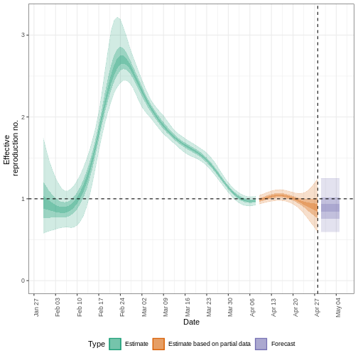
The uncertainty in the estimates increases through time. This is because estimates are informed by data in the past - within the delay periods. This difference in uncertainty is categorised into Estimate (green) utilises all data and Estimate based on partial data (orange) estimates that are based on less data (because infections that happened at the time are more likely to not have been observed yet) and therefore have increasingly wider intervals towards the date of the last data point. Finally, the Forecast (purple) is a projection ahead of time.

We can also visualise the growth rate estimate through time:

R

estimates$plots$growth_rate

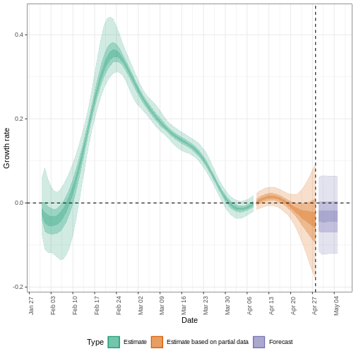
To extract a summary of the key transmission metrics at the latest date in the data:

R

summary(estimates)

OUTPUT

                        measure                estimate
                         <char>                  <char>
1:       New infections per day    7917 (4742 -- 12971)
2:   Expected change in reports       Likely decreasing
3:   Effective reproduction no.      0.96 (0.73 -- 1.2)
4:               Rate of growth -0.013 (-0.11 -- 0.076)
5: Doubling/halving time (days)       -52 (9.1 -- -6.6)

As these estimates are based on partial data, they have a wide uncertainty interval.

From the summary of our analysis we see that the expected change in reports is Likely decreasing with the estimated new infections 7917 (4742 – 12971).
The effective reproduction number $R_t$ estimate (on the last date of the data) is 0.96 (0.73 – 1.2).
The exponential growth rate of case numbers is -0.013 (-0.11 – 0.076).
The doubling time (the time taken for case numbers to double) is -52 (9.1 – -6.6).

`Expected change in reports`

A factor describing the expected change in reports based on the posterior probability that $R_t < 1$.

Probability ($p$)	Expected change
$p < 0.05$	Increasing
$0.05 \leq p< 0.4$	Likely increasing
$0.4 \leq p< 0.6$	Stable
$0.6 \leq p < 0.95$	Likely decreasing
$0.95 \leq p \leq 1$	Decreasing

Credible intervals

In all EpiNow2 output figures, shaded regions reflect 90%, 50%, and 20% credible intervals in order from lightest to darkest.

Checklist

EpiNow2 can be used to estimate transmission metrics from case data at any time in the course of an outbreak. The reliability of these estimates depends on the quality of the data and appropriate choice of delay distributions. In the next tutorial we will learn how to make forecasts and investigate some of the additional inference options available in EpiNow2.

How does {EpiNow2} work?

{EpiNow2} contains different models for how infections arise. One of the main models that is used in the default configuration is the Renewal equation model. If you want to gain familiarity with it and learn how delays are accounted for when estimating $R_t$, you can read the episode on Introduction to the Renewal equation in the “More Resources” section of this tutorial’s website.

Challenge

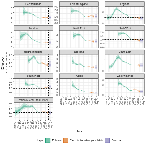
Quantify geographical heterogeneity

The outbreak data of the start of the COVID-19 pandemic from the United Kingdom from the R package incidence2 includes the region in which the cases were recorded. To find regional estimates of the effective reproduction number and cases, we must format the data to have three columns:

date: the date,
region: the region,
confirm: number of disease reports (confirm) for a region on a given date.

Generate regional Rt estimates from the incidence2::covidregionaldataUK data frame by:

use incidence2 to convert aggregated data to incidence data by the variable region,
keep the first 90 dates for all regions,
estimate the Rt per region using the defined generation time and delays in this episode.

R

regional_cases <- incidence2::covidregionaldataUK %>%
  # use {tidyr} to preprocess missing values
  tidyr::replace_na(base::list(cases_new = 0))

Give me a hint

To wrangle data, you can:

R

regional_cases <- incidence2::covidregionaldataUK %>%
  # use {tidyr} to preprocess missing values
  tidyr::replace_na(base::list(cases_new = 0)) %>%
  # use {incidence2} to convert aggregated data to incidence data
  incidence2::incidence(
    date_index = "date",
    groups = "region",
    counts = "cases_new",
    count_values_to = "confirm",
    date_names_to = "date",
    complete_dates = TRUE
  ) %>%
  dplyr::select(-count_variable) %>%
  dplyr::filter(date < ymd(20200301))

To learn how to do the regional estimation of Rt, read the Get started vignette section on regional_epinow() at https://epiforecasts.io/EpiNow2/articles/EpiNow2.html#regional_epinow

Show me the solution

To find regional estimates, we use the same inputs as epinow() to the function regional_epinow():

R

estimates_regional <- EpiNow2::regional_epinow(
  # cases
  data = regional_cases,
  # delays
  generation_time = EpiNow2::generation_time_opts(generation_time_fixed),
  delays = EpiNow2::delay_opts(incubation_period_fixed + reporting_delay_fixed),
  # prior
  rt = rt_prior
)

Plot the results with:

R

estimates_regional$summary$summarised_results$table

estimates_regional$summary$plots$R

Key Points

Transmission metrics can be estimated from case data after accounting for delays
Uncertainty can be accounted for in delay distributions

Probability (\(p\))	Expected change
\(p < 0.05\)	Increasing
\(0.05 \leq p< 0.4\)	Likely increasing
\(0.4 \leq p< 0.6\)	Stable
\(0.6 \leq p < 0.95\)	Likely decreasing
\(0.95 \leq p \leq 1\)	Decreasing

Quantifying transmission

Overview

Questions

Objectives

Prerequisites

Reminder: the Effective Reproduction Number, \(R_t\)

Introduction

R

The double-colon

Instructor Note

Bayesian inference

Instructor Note

Delay distributions and case data

Case data

R

OUTPUT

R

Show details

R

R

R

OUTPUT

Delay distributions

Delays and data

Incubation period distribution

R

OUTPUT

R

Why a gamma distribution?

Including distribution uncertainty

R

OUTPUT

R

Reporting delays

R

Show details

R

R

Show details

R

OUTPUT

OUTPUT

Generation time

R

Finding estimates

R

Bayesian inference using Stan

R

Checklist

R

R

Do not wait for this to continue

R

Results

R

R

R

OUTPUT

Expected change in reports

Credible intervals

Checklist

How does {EpiNow2} work?

Challenge

Challenge

R

Give me a hint

R

Show me the solution

R

R

Key Points

`Expected change in reports`