Instructor Notes
Instructor notes
Access epidemiological delay distributions
Instructor Note
Early models for COVID-19 used parameters from other coronaviruses. https://www.thelancet.com/article/S1473-3099(20)30144-4/fulltext
Instructor Note
The objective of the assessment above is to assess the interpretation of a larger or shorter generation time.
Instructor Note
R
# ebola serial interval
ebola_serial <-
  epiparameter::epiparameter_db(
    disease = "ebola",
    epi_name = "serial",
    single_epiparameter = TRUE
  )
OUTPUT
Using WHO Ebola Response Team, Agua-Agum J, Ariyarajah A, Aylward B, Blake I,
Brennan R, Cori A, Donnelly C, Dorigatti I, Dye C, Eckmanns T, Ferguson
N, Formenty P, Fraser C, Garcia E, Garske T, Hinsley W, Holmes D,
Hugonnet S, Iyengar S, Jombart T, Krishnan R, Meijers S, Mills H,
Mohamed Y, Nedjati-Gilani G, Newton E, Nouvellet P, Pelletier L,
Perkins D, Riley S, Sagrado M, Schnitzler J, Schumacher D, Shah A, Van
Kerkhove M, Varsaneux O, Kannangarage N (2015). "West African Ebola
Epidemic after One Year — Slowing but Not Yet under Control." _The New
England Journal of Medicine_. doi:10.1056/NEJMc1414992
<https://doi.org/10.1056/NEJMc1414992>..
To retrieve the citation use the 'get_citation' function
R
ebola_serial
OUTPUT
Disease: Ebola Virus Disease
Pathogen: Ebola Virus
Epi Parameter: serial interval
Study: WHO Ebola Response Team, Agua-Agum J, Ariyarajah A, Aylward B, Blake I,
Brennan R, Cori A, Donnelly C, Dorigatti I, Dye C, Eckmanns T, Ferguson
N, Formenty P, Fraser C, Garcia E, Garske T, Hinsley W, Holmes D,
Hugonnet S, Iyengar S, Jombart T, Krishnan R, Meijers S, Mills H,
Mohamed Y, Nedjati-Gilani G, Newton E, Nouvellet P, Pelletier L,
Perkins D, Riley S, Sagrado M, Schnitzler J, Schumacher D, Shah A, Van
Kerkhove M, Varsaneux O, Kannangarage N (2015). "West African Ebola
Epidemic after One Year — Slowing but Not Yet under Control." _The New
England Journal of Medicine_. doi:10.1056/NEJMc1414992
<https://doi.org/10.1056/NEJMc1414992>.
Distribution: gamma (days)
Parameters:
  shape: 2.188
  scale: 6.490
R
# get the sd
ebola_serial$summary_stats$sd
OUTPUT
[1] 9.6R
# get the sample_size
ebola_serial$metadata$sample_size
OUTPUT
[1] 305Try to visualise this distribution using plot().
Also, explore all the other nested elements within the
<epiparameter> object.
Share about:
- What elements do you find useful for your analysis?
- What other elements would you like to see in this object? How?
Instructor Note
An interesting element is the method_assess nested
entry, which refers to the methods used by the study authors to assess
for bias while estimating the serial interval distribution.
R
covid_serialint$method_assess
OUTPUT
$censored
[1] TRUE

$right_truncated
[1] TRUE

$phase_bias_adjusted
[1] FALSE
We will explore these concepts in the following episodes!
Instructor Note
In the context of user interfaces and graphical user interfaces (GUIs), like the Distribution Zoo shiny app, a slider is a graphical control element that allows users to adjust a value by moving a handle along a track or bar. Conceptually, it provides a way to select a numeric value within a specified range by visually sliding or dragging a pointer (the handle) along a continuous axis.
Quantifying transmission
Instructor Note
This tutorial illustrates the usage of epinow() to
estimate the time-varying reproduction number and infection times.
Learners should understand the necessary inputs to the model and the
limitations of the model output.
Instructor Note
Refer to the prior probability distribution and the posterior probability distribution.
In the “Expected change in reports”
callout, by “the posterior probability that \(R_t < 1\)”, we refer specifically to the
area
under the posterior probability distribution curve.
Use delay distributions in analysis
Instructor Note
You can access the reference documentation (help files) for these
functions with the triple-colon notation:
epiparameter:::
?epiparameter:::density.epiparameter()?epiparameter:::cdf.epiparameter()?epiparameter:::quantile.epiparameter()?epiparameter:::generate.epiparameter()
Instructor Note
How to create a distribution plot?
From a maximum value with quantile(), we can create a
sequence of quantile values as a numeric vector and calculate
density() values for each:
R
# create a discrete distribution visualisation
# from a maximum value from the distribution
quantile(covid_serialint_discrete, p = 0.99) %>%
  # generate quantile values
  # as a sequence for each natural number
  seq(1L, to = ., by = 1L) %>%
  # coerce numeric vector to data frame
  as_tibble_col(column_name = "quantile_values") %>%
  mutate(
    # calculate density values
    # for each quantile in the density function
    density_values =
      density(
        x = covid_serialint_discrete,
        at = quantile_values
      )
  ) %>%
  # create plot
  ggplot(
    aes(
      x = quantile_values,
      y = density_values
    )
  ) +
  geom_col()
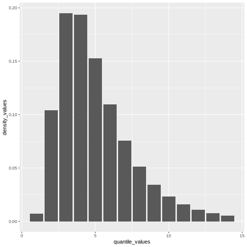
Remember: In infections with pre-symptomatic transmission, serial intervals can have negative values (Nishiura et al., 2020). When we use the serial interval to approximate the generation time we need to make this distribution with positive values only!
Instructor Note
We can stop the livecoding at this stage and move on with the practical.
Create a short-term forecast
Estimation of outbreak severity
Instructor Note
The periods are relevant: Period 1 – 15 days where CFR is zero to indicate this is due to no reported deaths; Period from Mar 15 – Apr 26 where CFR appears to be rising; Period Apr 30 – May 30 where the CFR estimate stabilises.
Instructor Note
We can showcase this last bias using the concept
described in this {cfr} vignette.
Instructor Note
There is almost one month of difference.
Note that the estimate has considerable uncertainty at the beginning of the time series. After two weeks, the delay-adjusted CFR approaches the overall CFR estimate at the outbreak’s end.
Is this pattern similar to other outbreaks? We can use the data sets in this episode’s challenges. We invite you to find it out!
Account for superspreading
Instructor Note
R
# estimate the probability of
# having a cluster size of 5, 10, or 25
# secondary cases from a primary case,
# given known reproduction number and
# dispersion parameter.
superspreading::proportion_cluster_size(
  R = ebola_offspring$estimate["mu"],
  k = ebola_offspring$estimate["size"],
  cluster_size = c(5, 10, 25)
)
OUTPUT
          R         k prop_5 prop_10 prop_25
1 0.3675993 0.8539443  2.64%      0%      0%
The probability of having clusters of five people is 1.8%. At this stage, given this offspring distribution parameters, a backward strategy may not increase the probability of contain and quarantine more onward cases.
Simulate transmission chains
Instructor Note
The function to generate random number from an
<epiparameter> class object can also accept this
notation:
R
as.function(x = serial_interval, func_type = "generate")
Instructor Note
R
# load packages -----------------------------------------------------------

library(epiparameter)
library(tidyverse)

# delays ------------------------------------------------------------------

mpox_offspring_epiparam <- epiparameter::epiparameter_db(
  disease = "mpox",
  epi_name = "offspring",
  single_epiparameter = TRUE
)

mpox_offspring <- epiparameter::get_parameters(mpox_offspring_epiparam)

mpox_serialint <- epiparameter::epiparameter_db(
  disease = "mpox",
  epi_name = "serial interval",
  single_epiparameter = TRUE
)

# iterate -----------------------------------------------------------------

# Set seed for random number generator
set.seed(33)

simulated_chains_mpox <- epichains::simulate_chains(
  n_chains = 1000,
  statistic = "size",
  offspring_dist = rnbinom,
  mu = mpox_offspring["mean"],
  size = mpox_offspring["dispersion"],
  generation_time = function(x) generate(x = mpox_serialint, times = x)
)

# visualize ---------------------------------------------------------------

# daily aggregate of cases
simulated_chains_mpox_day <- simulated_chains_mpox %>%
  # use data.frame output from <epichains> object
  as_tibble() %>%
  # Count the daily number of cases in each chain
  mutate(day = ceiling(time)) %>%
  count(chain, day, name = "cases") %>%
  # Calculate the cumulative number of cases for each chain
  group_by(chain) %>%
  mutate(cumulative_cases = cumsum(cases)) %>%
  ungroup()

# Visualize transmission chains by cumulative cases
simulated_chains_mpox_day %>%
  # Create grouped chain trajectories
  ggplot(aes(x = day, y = cumulative_cases, group = chain)) +
  geom_line(color = "black", alpha = 0.25, show.legend = FALSE) +
  # Define a 100-case threshold
  geom_hline(aes(yintercept = 100), lty = 2) +
  labs(x = "Day", y = "Cumulative cases")
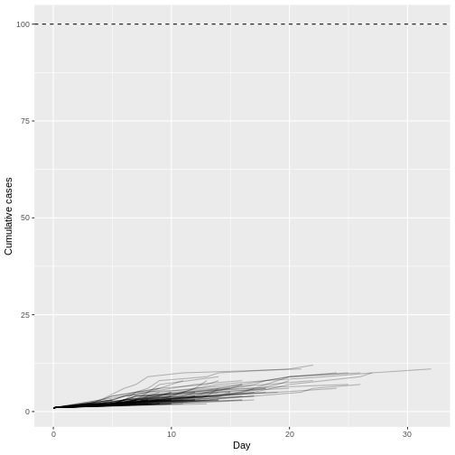
Assuming a Monkey pox outbreak with \(R\) = 0.32 and \(k\) = 0.58, there is no trajectory among 1000 simulations that reach more than 100 infected cases. Compared to MERS (\(R\) = 0.6 and \(k\) = 0.02).
Instructor Note
R
# load packages ---------------------------
library(epichains)
library(epiparameter)
library(fitdistrplus)
library(tidyverse)
R
# fit a negative binomial distribution ------------------------------------

# Fitting a negative binomial distribution to the number of secondary cases
fit.cases <- fitdistrplus::fitdist(c0, "nbinom")
fit.cases
OUTPUT
Fitting of the distribution ' nbinom ' by maximum likelihood
Parameters:
      estimate Std. Error
size 0.1814260 0.03990278
mu   0.9537995 0.19812301
R
# serial interval parameters ----------------------------------------------

ebola_serialinter <- epiparameter::epiparameter_db(
  disease = "ebola",
  epi_name = "serial interval",
  single_epiparameter = TRUE
)

# simulate outbreak trajectories ------------------------------------------

# Set seed for random number generator
set.seed(645)
sim_multiple_chains <- epichains::simulate_chains(
  n_chains = 100,
  statistic = "size",
  offspring_dist = rnbinom,
  mu = fit.cases$estimate["mu"],
  size = fit.cases$estimate["size"],
  generation_time = function(x) generate(x = ebola_serialinter, times = x)
)

# summarise ----------------------------------------

summary(sim_multiple_chains)
OUTPUT
`epichains_summary` object

  [1]    9    1    2    1    1    4    1   20   14    1    1  131    1    2    1
 [16]    1    7    1    2 2889    1    1    1   13    3    1    1    1    1    1
 [31]    5    6    1    1    1    1    1    1    1    1    2    1    1    2    1
 [46]    1    1    1    1    1    1    1    1    1  335    1   11    3   24    6
 [61]    1    1    1    1    1    1    1    1    1    1    1    1    1    1  111
 [76]    1    1    1    1    1    1    2    1  544    1    1    1    3    1    2
 [91]    6    1    1    1    1    1    1    1 2091    1

 Simulated sizes:

Max: 2889
Min: 1
R
# visualize ----------------------------------------

sim_chains_aggregate <-
  sim_multiple_chains %>%
  # use data.frame output from <epichains> object
  as_tibble() %>%
  # Count the daily number of cases in each chain
  mutate(day = ceiling(time)) %>%
  count(chain, day, name = "cases") %>%
  # Calculate the cumulative number of cases for each chain
  group_by(chain) %>%
  mutate(cumulative_cases = cumsum(cases)) %>%
  ungroup()

sim_chains_aggregate %>%
  # Create grouped chain trajectories
  ggplot(aes(x = day, y = cumulative_cases, group = chain)) +
  geom_line() +
  # Define a 100-case threshold
  geom_hline(aes(yintercept = 100), lty = 2) +
  ylim(0, 100) +
  xlim(0, 100) +
  labs(x = "Day", y = "Cumulative cases")
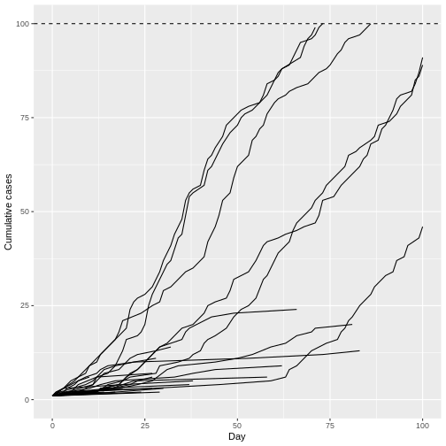
Remarkably, even with R0 less than 1 (R = 0.95) we can have potentially explosive outbreaks. The observed variation in individual infectiousness in Ebola means that although the probability of extinction is high, new index cases also have the potential for explosive regrowth of the epidemic.