Account for superspreading
Last updated on 2026-07-02 | Edit this page
Estimated time: 32 minutes
Overview
Questions
- How can we estimate individual-level variation in transmission (i.e. superspreading potential) from contact tracing data?
- What are the implications for variation in transmission for decision-making?
Objectives
- Estimate the distribution of onward transmission from infected individuals (i.e. offspring distribution) from outbreak data using epicontacts.
- Estimate the extent of individual-level variation (i.e. the dispersion parameter) of the offspring distribution using fitdistrplus.
- Estimate the proportion of transmission that is linked to ‘superspreading events’ using superspreading.
Learners should familiarise themselves with following concept dependencies before working through this tutorial:
Statistics: common probability distributions, particularly Poisson and negative binomial.
Epidemic theory: The reproduction number, R.
R packages installed: epicontacts, fitdistrplus, superspreading, outbreaks, tidyverse.
Install packages if they are not already installed
R
if (!base::require("pak")) install.packages("pak")
pak::pak(c("epicontacts", "fitdistrplus", "superspreading", "outbreaks", "tidyverse"))
If you have any error message, go to the main setup page.
Introduction
From smallpox to severe acute respiratory syndrome coronavirus 2 (SARS-CoV-2), some infected individuals spread infection to more people than others. Disease transmission is the result of a combination of biological and social factors, and these factors average out to some extent at the population level during a large epidemic. Hence researchers often use population averages to assess the potential for disease to spread. However, in the earlier or later phases of an outbreak, individual differences in infectiousness can be more important. In particular, they increase the chance of superspreading events (SSEs), which can ignite explosive epidemics and also influence the chances of controlling transmission (Lloyd-Smith et al., 2005).
The basic reproduction number, \(R_{0}\), measures the average number of cases caused by one infectious individual in a entirely susceptible population. Estimates of \(R_{0}\) are useful for understanding the average dynamics of an epidemic at the population-level, but can obscure considerable individual variation in infectiousness. This was highlighted during the global emergence of SARS-CoV-2 by numerous ‘superspreading events’ in which certain infectious individuals generated unusually large numbers of secondary cases (Leclerc et al., 2020).
In this tutorial, we are going to quantify individual variation in transmission, and hence estimate the potential for superspreading events. Then we are going to use these estimates to explore the implications of superspreading for contact tracing interventions.
We are going to use data from the outbreaks package, manage the linelist and contacts data using epicontacts, and estimate distribution parameters with fitdistrplus. Lastly, we are going to use superspreading to explore the implications of variation in transmission for decision-making.
We’ll use the pipe %>% to connect some of the
functions from these packages, so let’s also call the
tidyverse package.
R
library(outbreaks)
library(epicontacts)
library(fitdistrplus)
library(superspreading)
library(tidyverse)
The double-colon
The double-colon :: in R lets you call a specific
function from a package without loading the entire package into the
current environment. The package must be installed.
For example, dplyr::filter(data, condition) uses
filter() from the dplyr package.
This help us remember package functions and avoid namespace conflicts.
The individual reproduction number
The individual reproduction number is defined as the number of secondary cases caused by a particular infected individual.
Early in an outbreak we can use contact data to reconstruct transmission chains (i.e. who infected whom) and calculate the number of secondary cases generated by each individual. This reconstruction of linked transmission events from contact data can provide an understanding about how different individuals have contributed to transmission during an epidemic (Cori et al., 2017).
Let’s practice this using the mers_korea_2015 linelist
and contact data from the outbreaks package and integrate
them with the epicontacts package to calculate the
distribution of secondary cases during the 2015 MERS-CoV outbreak in
South Korea (Campbell,
2022):
R
## first, make an epicontacts object
epi_contacts <-
  epicontacts::make_epicontacts(
    linelist = outbreaks::mers_korea_2015$linelist,
    contacts = outbreaks::mers_korea_2015$contacts,
    directed = TRUE
  )
With the argument directed = TRUE we configure a
directed graph. These directions incorporate our hypothesis of the
infector-infectee pair: from the probable source
patient to the secondary case.
R
# visualise contact network
plot(epi_contacts)
Contact data from a transmission chain can provide information on
which infected individuals came into contact with others. We expect to
have the infector (from) and the infectee (to)
plus additional columns of variables related to their contact, such as
location (exposure) and date of contact.
Following tidy data principles, the observation unit in our contact data frame is the infector-infectee pair. Although one infector can infect multiple infectees, from contact tracing investigations we may record contacts linked to more than one infector (e.g. within a household). But we should expect to have unique infector-infectee pairs, because typically each infected person will have acquired the infection from one other.
To ensure these unique pairs, we can check on replicates for infectees:
R
# no infector-infectee pairs are replicated
epi_contacts %>%
  purrr::pluck("contacts") %>%
  dplyr::group_by(to) %>%
  dplyr::filter(dplyr::n() > 1)
OUTPUT
# A tibble: 5 × 4
# Groups:   to [2]
  from  to     exposure       diff_dt_onset
  <chr> <chr>  <fct>                  <int>
1 SK_16 SK_107 Emergency room            17
2 SK_87 SK_107 Emergency room             2
3 SK_14 SK_39  Hospital room             16
4 SK_11 SK_39  Hospital room             13
5 SK_12 SK_39  Hospital room             12
Our goal is to get the number of secondary cases caused by the observed infected individuals. In the contact data frame, when each infector-infectee pair is unique, the number of rows per infector corresponds to the number of secondary cases generated by that individual.
R
# count secondary cases per infector in contacts
epi_contacts %>%
  purrr::pluck("contacts") %>%
  dplyr::count(from, name = "secondary_cases")
OUTPUT
     from secondary_cases
1    SK_1              26
2   SK_11               1
3  SK_118               1
4   SK_12               1
5  SK_123               1
6   SK_14              38
7   SK_15               4
8   SK_16              21
9    SK_6               2
10  SK_76               2
11  SK_87               1
But this output only contains the number of secondary cases for
reported infectors in the contact data, not for all the
individuals in the whole <epicontacts> object.
Instead, from epicontacts we can use the function
epicontacts::get_degree(). The argument
type = "out" gets the out-degree of each
node in the contact network from the
<epicontacts> class object. In a directed network,
the out-degree is the number of outgoing edges (infectees) emanating
from a node (infector) (Nykamp DQ,
accessed: 2025).
Also, the argument only_linelist = TRUE will only
include individuals in the linelist data frame. During outbreak
investigations, we expect a registry of all the
observed infected individuals in the linelist data. However, anyone not
linked with a potential infector or infectee will not appear in the
contact data. Thus, the argument only_linelist = TRUE will
protect us against missing this later set of individuals when counting
the number of secondary cases caused by all the observed infected
individuals. They will appear in the <integer> vector
output as 0 secondary cases.
R
# Count secondary cases per subject in contacts and linelist
all_secondary_cases <- epicontacts::get_degree(
  x = epi_contacts,
  type = "out",
  only_linelist = TRUE
)
At epicontacts::get_degree() we use the argument
only_linelist = TRUE. This is to count the number of
secondary cases caused by all the observed infected individuals, which
includes individuals in contacts and linelist data frames.
The assumption that “the linelist will include all individuals in contacts and linelist” may not work for all situations.
For example, if during the registry of observed infections, the
contact data included more subjects than the ones available in the
linelist data, then you need to consider only the individuals from the
contact data. In that situation, at
epicontacts::get_degree() we use the argument
only_linelist = FALSE.
Find here a printed reproducible example:
R
# Three subjects on linelist
sample_linelist <- tibble::tibble(
  id = c("id1", "id2", "id3")
)

# Four infector-infectee pairs with Five subjects in contact data
sample_contact <- tibble::tibble(
  from = c("id1","id1","id2","id4"),
  to = c("id2","id3","id4","id5")
)

# make an epicontacts object
sample_net <- epicontacts::make_epicontacts(
  linelist = sample_linelist,
  contacts = sample_contact,
  directed = TRUE
)

# count secondary cases per subject from linelist only
epicontacts::get_degree(x = sample_net, type = "out", only_linelist = TRUE)
#> id1 id2 id3
#>   2   1   0

# count secondary cases per subject from contact only
epicontacts::get_degree(x = sample_net, type = "out", only_linelist = FALSE)
#> id1 id2 id4 id3 id5
#>   2   1   1   0   0
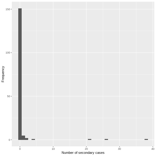
From a histogram of the all_secondary_cases object, we
can identify the individual-level variation in the
number of secondary cases. Three cases were related to more than 20
secondary cases, while the complementary cases with less than five or
zero secondary cases.
R
## plot the distribution
all_secondary_cases %>%
  tibble::enframe() %>%
  ggplot(aes(value)) +
  geom_histogram(binwidth = 1) +
  labs(
    x = "Number of secondary cases",
    y = "Frequency"
  )
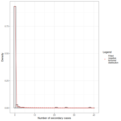
The number of secondary cases can be used to empirically estimate the offspring distribution, which is the number of secondary infections caused by each case. One candidate statistical distribution used to model the offspring distribution is the negative binomial distribution with two parameters:
Mean, which represents the \(R_{0}\), the average number of (secondary) cases produced by a single individual in an entirely susceptible population, and
Dispersion, expressed as \(k\), which represents the individual-level variation in transmission by single individuals.
From the histogram and density plot, we can identify that the offspring distribution is highly skewed or overdispersed. In this framework, the superspreading events (SSEs) are not arbitrary or exceptional, but simply realizations from the right-hand tail of the offspring distribution, which we can quantify and analyse (Lloyd-Smith et al., 2005).
Terminology recap
- From linelist and contact-tracing data, we calculate the number of secondary cases caused by the observed infected individuals.
- While \(R_{0}\) captures the average transmission in the population, the individual reproduction number represents the number of secondary infections caused by a specific infected individual, which varies between individuals.
- Because of stochastic effects in transmission, the number of secondary infections caused by each infection is statistically described by the offspring distribution.
- The empirical offspring distribution can be modeled using a negative binomial distribution with mean \(R_{0}\) and dispersion parameter \(k\), estimated from the observed number of secondary cases.
For occurrences of associated discrete events we can use Poisson or negative binomial discrete distributions.
In a Poisson distribution, mean is equal to variance. But when variance is higher than the mean, this is called overdispersion. In biological applications, overdispersion occurs and so a negative binomial may be worth considering as an alternative to Poisson distribution.
The negative binomial distribution is specially useful for discrete data over an unbounded positive range whose sample variance exceeds the sample mean. In such terms, the observations are overdispersed with respect to a Poisson distribution, for which the mean is equal to the variance.
In epidemiology, the negative binomial distribution has been used to model disease transmission for infectious diseases where the likely number of onward infections may vary considerably from individual to individual and from setting to setting, capturing all variation in infectious histories of individuals, including properties of the biological (i.e. degree of viral shedding) and environmental circumstances (e.g. type and location of contact).
Challenge
Calculate the distribution of secondary cases for Ebola using the
ebola_sim_clean object from outbreaks
package.
- Is the offspring distribution of Ebola skewed or overdispersed?
⚠️ Optional step: This dataset has 5829 cases.
Running plot(<epicontacts>) may take several minutes
and use significant memory for large outbreaks such as the Ebola
linelist. If you’re on an older or slower computer, you can skip this
step.
R
## first, make an epicontacts object
ebola_contacts <-
  epicontacts::make_epicontacts(
    linelist = outbreaks::ebola_sim_clean$linelist,
    contacts = outbreaks::ebola_sim_clean$contacts,
    directed = TRUE
  )

# count secondary cases per subject in contacts and linelist
ebola_secondary <- epicontacts::get_degree(
  x = ebola_contacts,
  type = "out",
  only_linelist = TRUE
)

## plot the distribution
ebola_secondary %>%
  tibble::enframe() %>%
  ggplot(aes(value)) +
  geom_histogram(binwidth = 1) +
  labs(
    x = "Number of secondary cases",
    y = "Frequency"
  )
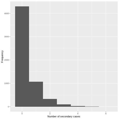
From a visual inspection, the distribution of secondary cases for the
Ebola data set in ebola_sim_clean shows an skewed
distribution with secondary cases equal or lower than 6. We need to
complement this observation with a statistical analysis to evaluate for
overdispersion.
Estimate the dispersion parameter
To empirically estimate the dispersion parameter \(k\), we could fit a negative binomial distribution to the number of secondary cases.
We can fit distributions to data using the fitdistrplus package, which provides maximum likelihood estimates.
R
library(fitdistrplus)
R
## fit distribution
offspring_fit <- all_secondary_cases %>%
  fitdistrplus::fitdist(distr = "nbinom")

offspring_fit
OUTPUT
Fitting of the distribution ' nbinom ' by maximum likelihood
Parameters:
       estimate  Std. Error
size 0.02039807 0.007278299
mu 0.60452947 0.337893199Name of parameters
From the fitdistrplus output:
- The
sizeobject refers to the estimated dispersion parameter \(k\), and - The
muobject refers to the estimated mean, which represents the \(R_{0}\),
From the number secondary cases distribution we estimated a dispersion parameter \(k\) of 0.02, with a 95% Confidence Interval from 0.006 to 0.035. As the value of \(k\) is significantly lower than one, we can conclude that there is considerable potential for superspreading events.
We can overlap the estimated density values of the fitted negative binomial distribution and the histogram of the number of secondary cases:
Individual-level variation in transmission
The individual-level variation in transmission is defined by the relationship between the mean (\(R_{0}\)) and dispersion (\(k\)), which together define the variance of a negative binomial distribution.
The negative binomial model has \(variance = R_{0}(1+\frac{R_{0}}{k})\), so smaller values of \(k\) indicate greater variance and, consequently, greater individual-level variation in transmission.
\[\uparrow variance = R_{0}(1+\frac{R_{0}}{\downarrow k})\]
When \(k\) approaches infinity (\(k \rightarrow \infty\)) the variance equals the mean (because \(\frac{R_{0}}{\infty}=0\)). This makes the conventional Poisson model an special case of the negative binomial model.
Challenge
From the previous challenge, use the distribution of secondary cases
from the ebola_sim_clean object from
outbreaks package.
Fit a negative binomial distribution to estimate the mean and dispersion parameter of the offspring distribution. Try to estimate the uncertainty of the dispersion parameter from the Standard Error to 95% Confidence Intervals.
- Does the estimated dispersion parameter of Ebola provide evidence of an individual-level variation in transmission?
Review how we fitted a negative binomial distribution using the
fitdistrplus::fitdist() function.
R
ebola_offspring <- ebola_secondary %>%
  fitdistrplus::fitdist(distr = "nbinom")

ebola_offspring
OUTPUT
Fitting of the distribution ' nbinom ' by maximum likelihood
Parameters:
      estimate  Std. Error
size 0.8539443 0.072505326
mu   0.3675993 0.009497097
R
## extract the "size" parameter
ebola_mid <- ebola_offspring$estimate[["size"]]

## calculate the 95% confidence intervals using the
## standard error estimate and
## the 0.025 and 0.975 quantiles of the normal distribution.

ebola_lower <- ebola_mid + ebola_offspring$sd[["size"]] * qnorm(0.025)
ebola_upper <- ebola_mid + ebola_offspring$sd[["size"]] * qnorm(0.975)

# ebola_mid
# ebola_lower
# ebola_upper
From the number secondary cases distribution we estimated a dispersion parameter \(k\) of 0.85, with a 95% Confidence Interval from 0.71 to 1.
For dispersion parameter estimates higher than one we get low distribution variance, hence, low individual-level variation in transmission.
But does this mean that the secondary case distribution does not have superspreading events (SSEs)? You will later find one additional challenge: How do you define an SSE threshold for Ebola?
We can use the maximum likelihood estimates from
fitdistrplus to compare different models and assess fit
performance using estimators like the AIC and BIC. Read further in the
vignette on Estimate
individual-level transmission and use the
superspreading helper function ic_tbl() for
this!
The dispersion parameter across diseases
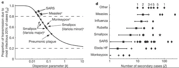
Research into sexually transmitted and vector-borne diseases has previously suggested a ‘20/80’ rule, with 20% of individuals contributing at least 80% of the transmission potential (Woolhouse et al., 1997).
On its own, the dispersion parameter \(k\) is hard to interpret intuitively, and hence converting into proportional summary can enable easier comparison. When we consider a wider range of pathogens, we can see there is no hard and fast rule for the percentage that generates 80% of transmission, but variation does emerge as a common feature of infectious diseases
When the 20% most infectious cases contribute to the 80% of transmission (or more), there is a high individual-level variation in transmission, with a highly overdispersed offspring distribution (\(k<0.1\)), e.g., SARS-1.
When the 20% most infectious cases contribute to the ~50% of transmission, there is a low individual-level variation in transmission, with a moderately dispersed offspring distribution (\(k > 0.1\)), e.g. Pneumonic Plague.
Controlling superspreading with contact tracing
During an outbreak, it is common to try and reduce transmission by identifying people who have come into contact with an infected person, then quarantine them in case they subsequently turn out to be infected. Such contact tracing can be deployed in multiple ways. ‘Forward’ contact tracing targets downstream contacts who may have been infected by a newly identifed infection (i.e. the ‘index case’). ‘Backward’ tracing instead tracks the upstream primary case who infected the index case (or a setting or event at which the index case was infected), for example by retracing history of contact to the likely point of exposure. This makes it possible to identify others who were also potentially infected by this earlier primary case.
In the presence of individual-level variation in transmission, i.e., with an overdispersed offspring distribution, if this primary case is identified, a larger fraction of the transmission chain can be detected by forward tracing each of the contacts of this primary case (Endo et al., 2020).
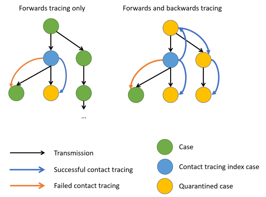
When there is evidence of individual-level variation (i.e. overdispersion), often resulting in so-called superspreading events, a large proportion of infections may be linked to a small proportion of original clusters. As a result, finding and targeting originating clusters in combination with reducing onwards infection may substantially enhance the effectiveness of tracing methods (Endo et al., 2020).
Empirical evidence focused on evaluating the efficiency of backward tracing led to 42% more cases identified than forward tracing supporting its implementation when rigorous suppression of transmission is justified (Raymenants et al., 2022).
Probability of cases in a given cluster
Using superspreading, we can estimate the probability of having a cluster of secondary infections caused by a primary case identified by backward tracing of size \(X\) or larger (Endo et al., 2020).
R
# Set seed for random number generator
set.seed(33)

# estimate the probability of
# having a cluster size of 5, 10, or 25
# secondary cases from a primary case,
# given known reproduction number and
# dispersion parameter.
superspreading::proportion_cluster_size(
  R = offspring_fit$estimate["mu"],
  k = offspring_fit$estimate["size"],
  cluster_size = c(5, 10, 25)
)
OUTPUT
          R          k prop_5 prop_10 prop_25
1 0.6045295 0.02039807  87.9%   74.6%   46.1%
Even though we have an \(R<1\), a highly overdispersed offspring distribution (\(k=0.02\)) means that if we detect a new case, there is a 46.1% probability they originated from a cluster of 25 infections or more. Hence, by following a backwards strategy, contact tracing efforts will increase the probability of successfully contain and quarantining this large number of earlier infected individuals, rather than simply focusing on the new case, who is likely to have infected nobody (because \(k\) is very small).
We can also use this number to prevent gatherings of a certain size to reduce the epidemic by preventing potential superspreading events. Interventions can target to reduce the reproduction number in order to reduce the probability of having clusters of secondary cases.
Backward contact tracing for Ebola
Use the Ebola estimated parameters for ebola_sim_clean
object from outbreaks package.
Calculate the probability of having a cluster of secondary infections caused by a primary case identified by backward tracing of size 5, 10, 15 or larger.
Would implementing a backward strategy at this stage of the Ebola outbreak increase the probability of containing and quarantining more onward cases?
Review how we estimated the probability of having clusters of a fixed
size, given an offspring distribution mean and dispersion parameters,
using the superspreading::proportion_cluster_size()
function.
R
# estimate the probability of
# having a cluster size of 5, 10, or 25
# secondary cases from a primary case,
# given known reproduction number and
# dispersion parameter.
superspreading::proportion_cluster_size(
  R = ebola_offspring$estimate["mu"],
  k = ebola_offspring$estimate["size"],
  cluster_size = c(5, 10, 25)
)
OUTPUT
          R         k prop_5 prop_10 prop_25
1 0.3675993 0.8539443  2.64%      0%      0%
The probability of having clusters of five people is 1.8%. At this stage, given this offspring distribution parameters, a backward strategy may not increase the probability of contain and quarantine more onward cases.
Challenges
Does Ebola have any superspreading event?
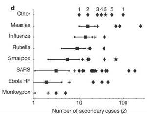
‘Superspreading events’ can mean different things to different people, so Lloyd-Smith et al., 2005 proposed a general protocol for defining a superspreading event (SSE). If the number of secondary infections caused by each case, \(Z\), follows a negative binomial distribution (\(R, k\)):
- We define an SSE as any infected individual who infects more than \(Z(n)\) others, where \(Z(n)\) is the nth percentile of the \(Poisson(R)\) distribution.
- A 99th-percentile SSE is then any case causing more infections than would occur in 99% of infectious histories in a homogeneous population
Using the corresponding distribution function, estimate the SSE
threshold to define a SSE for the Ebola offspring distribution estimates
for the ebola_sim_clean object from
outbreaks package.
In a Poisson distribution, the lambda or rate parameter are equal to the estimated mean from a negative binomial distribution. You can explore this in The distribution zoo shiny app.
To get the quantile value for the 99th-percentile we need to use the
density
function for the Poisson distribution dpois().
R
# get mean
ebola_mu_mid <- ebola_offspring$estimate["mu"]

# get 99th-percentile from poisson distribution
# with mean equal to mu
stats::qpois(
  p = 0.99,
  lambda = ebola_mu_mid
)
OUTPUT
[1] 2Compare this values with the ones reported by Lloyd-Smith et al., 2005. See figure below:
Expected proportion of transmission
What is the proportion of cases responsible for 80% of transmission?
Use superspreading and compare the estimates for MERS using the offspring distributions parameters from this tutorial episode, with SARS-1 and Ebola offspring distributions parameter accessible via the epiparameter R package.
To use superspreading::proportion_transmission() we
recommend to read the Estimate
what proportion of cases cause a certain proportion of transmission
reference manual.
Currently, epiparameter has offspring distributions
for SARS, Smallpox, Mpox, Pneumonic Plague, Hantavirus Pulmonary
Syndrome, Ebola Virus Disease. Let’s access the offspring distribution
mean and dispersion parameters for SARS-1:
R
# Load parameters
sars <- epiparameter::epiparameter_db(
  disease = "SARS",
  epi_name = "offspring distribution",
  single_epiparameter = TRUE
)
sars_params <- epiparameter::get_parameters(sars)
sars_params
OUTPUT
      mean dispersion
1.63 0.16 R
#' estimate for ebola --------------

ebola_epiparameter <- epiparameter::epiparameter_db(
  disease = "Ebola",
  epi_name = "offspring distribution",
  single_epiparameter = TRUE
)
ebola_params <- epiparameter::get_parameters(ebola_epiparameter)
ebola_params
OUTPUT
      mean dispersion
       1.5        5.1
R
# estimate
# proportion of cases that
# generate 80% of transmission
superspreading::proportion_transmission(
  R = ebola_params[["mean"]],
  k = ebola_params[["dispersion"]],
  prop_transmission = 0.8
)
OUTPUT
    R   k prop_80
1 1.5 5.1   43.2%
R
#' estimate for sars --------------

# estimate
# proportion of cases that
# generate 80% of transmission
superspreading::proportion_transmission(
  R = sars_params[["mean"]],
  k = sars_params[["dispersion"]],
  prop_transmission = 0.8
)
OUTPUT
     R    k prop_80
1 1.63 0.16     13%
R
#' estimate for mers --------------

# estimate
# proportion of cases that
# generate 80% of transmission
superspreading::proportion_transmission(
  R = offspring_fit$estimate["mu"],
  k = offspring_fit$estimate["size"],
  prop_transmission = 0.8
)
OUTPUT
          R          k prop_80
1 0.6045295 0.02039807   2.13%
MERS has the lowest percent of cases (2.1%) responsible of the 80% of the transmission, representative of highly overdispersed offspring distributions.
Ebola has the highest percent of cases (43%) responsible of the 80% of the transmission. This is representative of offspring distributions with high dispersion parameters.
inverse-dispersion?
The dispersion parameter \(k\) can be expressed differently across the literature.
- In the Wikipedia page for the negative binomial, this parameter is defined in its reciprocal form (refer to the variance equation).
- In the distribution zoo shiny app, the dispersion parameter \(k\) is named “Inverse-dispersion” but it is equal to parameter estimated in this episode. We invite you to explore this!
heterogeneity?
The individual-level variation in transmission is also referred as
the heterogeneity in the transmission or degree of heterogeneity in Lloyd-Smith et
al., 2005, heterogeneous infectiousness in Campbell
et al., 2018 when introducing the {outbreaker2}
package. Similarly, a contact network can store heterogeneous
epidemiological contacts as in the documentation of the
epicontacts package (Nagraj
et al., 2018).
Read these blog posts
The Tracing monkeypox article from the JUNIPER consortium showcases the usefulness of network models on contact tracing.
The Going viral post from Adam Kucharski shares insides from YouTube virality, disease outbreaks, and marketing campaigns on the conditions that spark contagion online.
- Use epicontacts to calculate the number of secondary cases cause by a particular individual from linelist and contact data.
- Use fitdistrplus to empirically estimate the offspring distribution from the number of secondary cases distribution.
- Use superspreading to estimate the probability of having clusters of a given size from primary cases and inform contact tracing efforts.