Analyzing demographic data with epiCo

epiCo’s demographic module is a tool for demographic descriptive analysis and risk assessment of epidemiological events in Colombia. Based on linelist data provided by the Colombian National Surveillance System (SIVIGILA) and demographic data from the Colombian National Administrative Department of Statistics (DANE).

The module allows you to:

• Consult and visualize the population pyramid of a municipality, department, or country for a year of interest.
• Consult the definitions of demographic variables such as ethnicities, special population groups, and occupational labels.
• Estimate the distribution of occupations reported in the line list according to the ISCO 88 Standard.
• Estimate the incidence rate of a municipality, department, or country.
• Calculate and visualize a relative age risk by normalizing the distribution of cases by the specific age structure of the location of interest.

In the following vignette, you will learn how to:

1. Navigate the Codification of the Political Administrative Division of Colombia (DIVIPOLA).
2. Consult, visualize, and interpret Colombian population pyramids at different administrative levels.
3. Interpret the demographic variables reported by the SIVIGILA (as ethnicities, special population groups, and occupational labels).
4. Understand the typical SIVIGILA epidemiological data.
5. Estimate weekly and monthly incidence rates for a municipality, department, or country.
6. Integrate the age distributions of cases with population pyramids to obtain an age-risk assessment for a disease.

1. Navigating the Codification of the Political Administrative Division of Colombia (DIVIPOLA)

DIVIPOLA is a standardized nomenclature designed by the DANE for the identification of territorial entities (departments, districts, and municipalities), non-municipalized areas, and populated centers by assigning a unique numerical code to each of these territorial units.

Colombia has:

• 32 Departments (Administrative Division Level 1)
• 1102 Municipalities (Administrative Division Level 2)
• 1 Island
• 18 Non-municipalized areas
• 6678 Populated centers

Two digits are used for the codification of departments, and five digits are used for the codification of municipalities (the first two being the department where they are located).

epiCo provides the complete list of departments and municipalities codes through a built-in dataset.

library(epiCo)
library(incidence)

data("divipola_table")

2. Population pyramids

epiCo provides a built-in dataset with the population projections of Colombia at the national, departmental, and municipality levels (provided by the DANE). These datasets contains the population projections from 2012 to 2024 for ages from 0 to 100 years. However, for the municipal projections it has the ages from 0 to over 85 years old.

Users can perform queries on this data by using the population_pyramid function, providing the DIVIPOLA code of the territory of interest and the year to consult.

ibague_code <- "73001" # DIVIPOLA code for the city of Ibagu<U+00E9>
year <- 2016 # Year to consult
ibague_pyramid_2016 <- population_pyramid(ibague_code, year) # Population
# pyramid (dataframe) for the city of Ibagu<U+00E9> in the year 2019
# dissagregated by sex
knitr::kable(ibague_pyramid_2016[1:5, ])

age	population	sex
0	15839	F
5	17539	F
10	20171	F
15	23059	F
20	22659	F

Definitions of age ranges and plotting are also provided for both: total number of individuals, or proportion of individuals

ibague_code <- "73001" # DIVIPOLA code for the city of Ibagué
year <- 2019 # Year to consult
age_range <- 5 # Age range or window
ibague_pyramid_2019 <- population_pyramid(ibague_code, year,
  range = age_range,
  sex = TRUE, total = TRUE,
  plot = TRUE
)

Population pyramid for the city of Ibagué in 2019

3. Demographic variables

Events of epidemiological relevance are reported to the SIVIGILA using an official notification form (see link).

epiCo provides a function to consult the dictionaries for the ethnicity categories, special population groups, and occupation codifications used by the SIVIGILA. As shown in the following example:

demog_data <- data.frame(
  id = c(0001, 002, 003, 004, 005, 006, 007, 008),
  ethnicity_label = c(3, 4, 2, 3, 3, 3, 2, 3),
  occupation_label = c(6111, 3221, 5113, 5133, 6111, 23, 25, 99),
  sex = c("F", "M", "F", "F", "M", "M", "F", "M"),
  stringsAsFactors = FALSE
)


ethnicities <- describe_ethnicity(demog_data$ethnicity_label)
knitr::kable(ethnicities)

code	description
2	They are communities that have their own ethnic and cultural identity; They are characterized by a nomadic tradition, and have their own language, which is Romanesque
3	Population located in the Archipelago of San Andres, Providencia and Santa Catalina, with Afro-Anglo-Antillean cultural roots, whose members have clearly differentiated sociocultural and linguistic traits from the rest of the Afro-Colombian population
4	Population located in the municipality of San Basilio de Palenque, department of Bolivar, where palenquero is spoken, a Creole language

occupations <- describe_occupation(
  isco_codes = demog_data$occupation_label,
  sex = demog_data$sex,
  plot = "treemap"
)
#> 2 codes are invalid.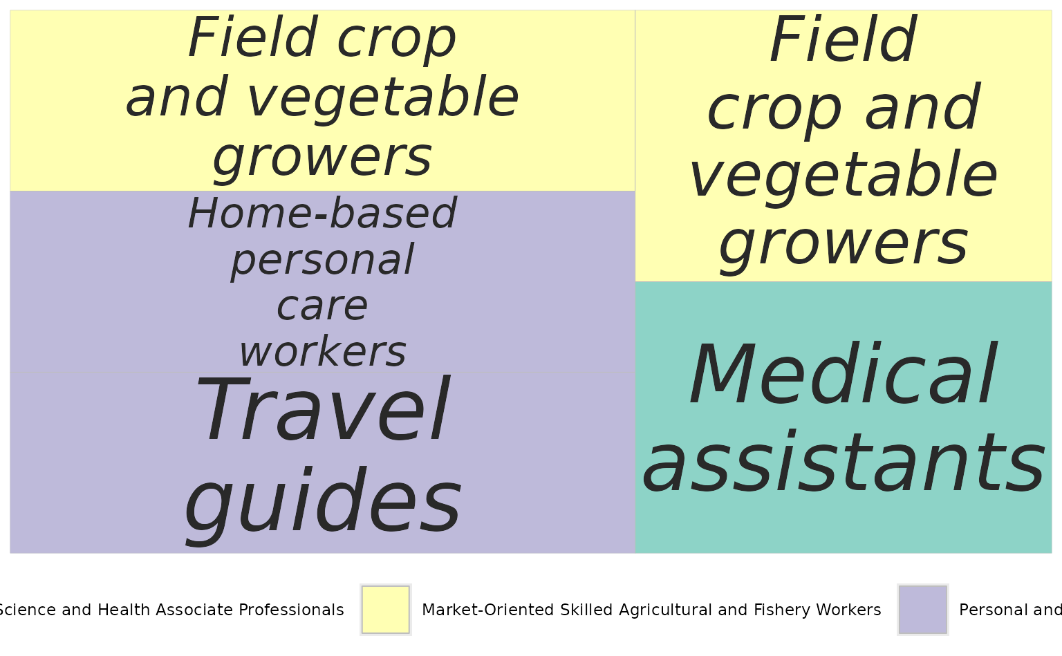

Treemap plot of the distribution of occupations reported in the line list

knitr::kable(occupations$data)

major	major_label	sub_major	sub_major_label	minor	minor_label	unit	unit_label	sex	count
5	Service Workers and Shop and Market Sales Workers	51	Personal and Protective Services Workers	511	Travel Attendants and Related Workers	5113	Travel guides	F	1
5	Service Workers and Shop and Market Sales Workers	51	Personal and Protective Services Workers	513	Personal Care and Related Workers	5133	Home-based personal care workers	F	1
6	Skilled Agricultural and Fishery Workers	61	Market-Oriented Skilled Agricultural and Fishery Workers	611	Market Gardeners and Crop Growers	6111	Field crop and vegetable growers	F	1
2	Professionals	23	Teaching Professionals	NA	NA	NA	NA	M	1
3	Technicians and Associate Professionals	32	Life Science and Health Associate Professionals	322	Modern Health Associate Professionals (Except Nursing)	3221	Medical assistants	M	1
6	Skilled Agricultural and Fishery Workers	61	Market-Oriented Skilled Agricultural and Fishery Workers	611	Market Gardeners and Crop Growers	6111	Field crop and vegetable growers	M	1
NA	NA	NA	NA	NA	NA	NA	NA	NA	2

4. Epidemiological data

epiCo is a tool that produces analyses based on epidemiological data extracted from SIVIGILA or provided by the user. epi_data is a built-in file that shows an example of the structure used by the package, which is the same as the one reported by SIVIGILA. This file contains the cases of all the municipalities in Tolima for the years 2015-2021.

The following analyses use the dengue cases reported in Tolima in 2019.

data("epi_data")

data_tolima <- epi_data[lubridate::year(epi_data$fec_not) == 2019, ]
knitr::kable(data_tolima[1:5, 4:12])

cod_mun_o	cod_pais_r	cod_dpto_r	cod_mun_r	cod_dpto_n	cod_mun_n	edad	sexo	per_etn
73001	170	73	73001	25	25307	11	F	6
73268	170	73	73268	73	73268	18	F	6
73200	170	73	73200	11	11001	13	M	6
73671	170	73	73671	73	73671	16	M	6
73671	170	73	73671	73	73671	15	M	6

5. Estimation of incidence rates

The incidence rate feature of epiCo requires the incidence package to produce a modified incidence object. Instead of a count vector (or matrix), it transforms the object to provide a rate element accounting for the number of cases in the time period divided by the total number of inhabitants in the specific region and year.

epiCo uses the DANE population projections as denominators; therefore, it is necessary to provide the administration level at which incidences are calculated.

incidence_object <- incidence(
  dates = data_tolima$fec_not,
  groups = data_tolima$cod_mun_o,
  interval = "1 epiweek"
)
incidence_rate_object <- incidence_rate(incidence_object, level = 2)
knitr::kable(incidence_rate_object$counts[1:5, 1:12])

73001	73024	73026	73030	73043	73055	73067	73124	73148	73152	73168	73200
12	1	1	0	0	0	1	0	0	0	1	1
12	0	1	1	0	1	0	0	1	0	16	0
17	1	1	0	0	1	2	0	0	0	4	0
15	0	1	0	0	3	0	0	2	0	10	0
23	0	1	0	0	1	0	0	0	0	15	0

If groups in the incidence object are not within the DIVIPOLA coding for municipalities (level 2) or departments (level 1), or a national estimation is intended (level 0), the function will not be able to estimate an incidence rate.

6. Estimation of risk by age group

Normalization of data is a key aspect of epidemiology. epiCo allows for the age distribution of cases and normalizes the epidemiological data with the age structure of a population. This normalization allows us to estimate the age risk of a disease according to the age structure of the general population in a municipality, department, or country in a certain year.

data_ibague <- data_tolima[data_tolima$cod_mun_o == 73001, ]

age_risk_data <- age_risk(
  age = data_ibague$edad,
  population_pyramid = ibague_pyramid_2019$data,
  sex = data_ibague$sexo, plot = TRUE
)

Age risk plot for the city of Ibagué in 2019