Use delay distributions in analysis
Last updated on 2024-06-18 | Edit this page
Estimated time: 30 minutes
Overview
Questions
- How to reuse delays stored in the
{epiparameter}library with my existing analysis pipeline?
Objectives
- Use distribution functions to continuous and discrete distributions
stored as
<epidist>objects. - Convert a continuous to a discrete distribution with
{epiparameter}. - Connect
{epiparameter}outputs with EpiNow2 inputs.
Prerequisites
- Complete tutorial Quantifying transmission
This episode requires you to be familiar with:
Data science : Basic programming with R.
Statistics : Probability distributions.
Epidemic theory : Epidemiological parameters, time periods, Effective reproductive number.
Introduction
{epiparameter} help us to choose one specific
set of epidemiological parameters from the literature, instead of
copy/pasting them by hand:
R
covid_serialint <-
  epiparameter::epidist_db(
    disease = "covid",
    epi_dist = "serial",
    author = "Nishiura",
    single_epidist = TRUE
  )
Now, we have an epidemiological parameter we can use in our analysis!
In the chunk below we replaced one of the summary
statistics inputs into EpiNow2::LogNormal()
R
generation_time <-
  EpiNow2::LogNormal(
    mean = covid_serialint$summary_stats$mean, # replaced!
    sd = covid_serialint$summary_stats$sd, # replaced!
    max = 20
  )
In this episode, we will use the distribution
functions that {epiparameter} provides to get a
maximum value (max) for this and any other package
downstream in your analysis pipeline!
Let’s load the {epiparameter} and EpiNow2
package. For EpiNow2, we’ll set 4 cores to be used in
parallel computations. We’ll use the pipe %>%, some
dplyr verbs and ggplot2, so let’s also
call to the tidyverse package:
R
library(epiparameter)
library(EpiNow2)
library(tidyverse)

withr::local_options(list(mc.cores = 4))
The double-colon
The double-colon :: in R let you call a specific
function from a package without loading the entire package into the
current environment.
For example, dplyr::filter(data, condition) uses
filter() from the dplyr package.
This help us remember package functions and avoid namespace conflicts.
Distribution functions
In R, all the statistical distributions have functions to access the following:
-
density(): Probability Density function (PDF), -
cdf(): Cumulative Distribution function (CDF), -
quantile(): Quantile function, and -
generate(): Random values from the given distribution.
Functions for the Normal distribution
If you need it, read in detail about the R probability functions for the normal distribution, each of its definitions and identify in which part of a distribution they are located!
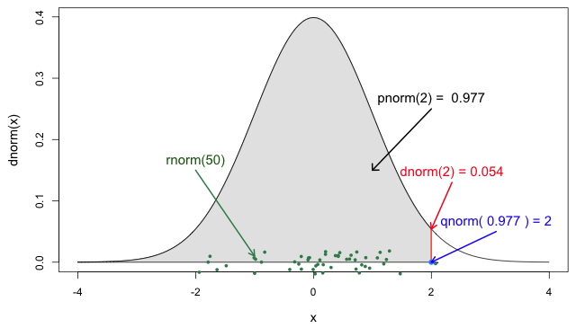
If you look at ?stats::Distributions, each type of
distribution has a unique set of functions. However,
{epiparameter} gives you the same four functions to access
each of the values above for any <epidist> object you
want!
R
# plot this to have a visual reference
plot(covid_serialint, day_range = 0:20)
R
# the density value at quantile value of 10 (days)
density(covid_serialint, at = 10)
OUTPUT
[1] 0.01911607R
# the cumulative probability at quantile value of 10 (days)
cdf(covid_serialint, q = 10)
OUTPUT
[1] 0.9466605R
# the quantile value (day) at a cumulative probability of 60%
quantile(covid_serialint, p = 0.6)
OUTPUT
[1] 4.618906R
# generate 10 random values (days) given
# the distribution family and its parameters
generate(covid_serialint, times = 10)
OUTPUT
 [1] 1.817744 2.013148 2.871411 1.560954 4.544691 7.315718 2.563274 6.472184
[9] 8.090210 6.302332Access to the reference documentation (Help files) for these
functions is accessible with the three double-colon notation:
epiparameter:::
?epiparameter:::density.epidist()?epiparameter:::cdf.epidist()?epiparameter:::quantile.epidist()?epiparameter:::generate.epidist()
Window for contact tracing and the serial interval
The serial interval is important in the optimisation of contact tracing since it provides a time window for the containment of a disease spread (Fine, 2003). Depending on the serial interval, we can evaluate the need to expand the number of days pre-onset to consider in the contact tracing to include more backwards contacts (Davis et al., 2020).
With the COVID-19 serial interval (covid_serialint)
calculate:
- How much more of the backward cases could be captured if the contact tracing method considered contacts up to 6 days pre-onset compared to 2 days pre-onset?
In Figure 5 from the R
probability functions for the normal distribution, the shadowed
section represents a cumulative probability of 0.997 for
the quantile value at x = 2.
R
plot(covid_serialint)
R
cdf(covid_serialint, q = 2)
OUTPUT
[1] 0.1111729R
cdf(covid_serialint, q = 6)
OUTPUT
[1] 0.7623645Given the COVID-19 serial interval:
A contact tracing method considering contacts up to 2 days pre-onset will capture around 11.1% of backward cases.
If this period is extended to 6 days pre-onset, this could include 76.2% of backward contacts.
If we exchange the question between days and cumulative probability to:
- When considering secondary cases, how many days following the symptom onset of primary cases can we expect 55% of symptom onset to occur?
R
quantile(covid_serialint, p = 0.55)
An interpretation could be:
- The 55% percent of the symptom onset of secondary cases will happen after 4.2 days after the symptom onset of primary cases.
Discretise a continuous distribution
We are getting closer to the end! EpiNow2::LogNormal()
still needs a maximum value (max).
One way to do this is to get the quantile value for the
distribution’s 99th percentile or 0.99 cumulative
probability. For this, we need access to the set of distribution
functions for our <epidist> object.
We can use the set of distribution functions for a
continuous distribution (as above). However, these values will
be continuous numbers. We can discretise the
continuous distribution stored in our <epidist>
object to get discrete values from a continuous distribution.
When we epiparameter::discretise() the continuous
distribution we get a discrete(-ized) distribution:
R
covid_serialint_discrete <-
  epiparameter::discretise(covid_serialint)

covid_serialint_discrete
OUTPUT
Disease: COVID-19
Pathogen: SARS-CoV-2
Epi Distribution: serial interval
Study: Nishiura H, Linton N, Akhmetzhanov A (2020). "Serial interval of novel
coronavirus (COVID-19) infections." _International Journal of
Infectious Diseases_. doi:10.1016/j.ijid.2020.02.060
<https://doi.org/10.1016/j.ijid.2020.02.060>.
Distribution: discrete lnorm
Parameters:
  meanlog: 1.386
  sdlog: 0.568
We identify this change in the Distribution: output line
of the <epidist> object. Double check this line:
Distribution: discrete lnormWhile for a continuous distribution, we plot the Probability Density Function (PDF), for a discrete distribution, we plot the Probability Mass Function (PMF):
R
# continuous
plot(covid_serialint)

# discrete
plot(covid_serialint_discrete)
To finally get a max value, let’s access the quantile
value of the 99th percentile or 0.99 probability of the
distribution with the prob_dist$q notation, similarly to
how we access the summary_stats values.
R
covid_serialint_discrete_max <-
  quantile(covid_serialint_discrete, p = 0.99)
Length of quarantine and incubation period
The incubation period distribution is a useful delay to assess the length of active monitoring or quarantine (Lauer et al., 2020). Similarly, delays from symptom onset to recovery (or death) will determine the required duration of health care and case isolation (Cori et al., 2017).
Calculate:
- Within what exact time frame do 99% of individuals exhibiting COVID-19 symptoms exhibit them after infection?
What delay distribution measures the time between infection and the onset of symptoms?
The probability functions for <epidist>
discrete distributions are the same that we used for
the continuous ones!
R
# plot to have a visual reference
plot(covid_serialint_discrete, day_range = 0:20)

# density value at quantile value 10 (day)
density(covid_serialint_discrete, at = 10)

# cumulative probability at quantile value 10 (day)
cdf(covid_serialint_discrete, q = 10)

# In what quantile value (days) do we have the 60% cumulative probability?
quantile(covid_serialint_discrete, p = 0.6)

# generate random values
generate(covid_serialint_discrete, times = 10)
R
covid_incubation <-
  epiparameter::epidist_db(
    disease = "covid",
    epi_dist = "incubation",
    single_epidist = TRUE
  )
OUTPUT
Using Linton N, Kobayashi T, Yang Y, Hayashi K, Akhmetzhanov A, Jung S, Yuan
B, Kinoshita R, Nishiura H (2020). "Incubation Period and Other
Epidemiological Characteristics of 2019 Novel Coronavirus Infections
with Right Truncation: A Statistical Analysis of Publicly Available
Case Data." _Journal of Clinical Medicine_. doi:10.3390/jcm9020538
<https://doi.org/10.3390/jcm9020538>..
To retrieve the citation use the 'get_citation' function
R
covid_incubation_discrete <- epiparameter::discretise(covid_incubation)

quantile(covid_incubation_discrete, p = 0.99)
OUTPUT
[1] 1999% of those who develop COVID-19 symptoms will do so within 16 days of infection.
Now, Is this result expected in epidemiological terms?
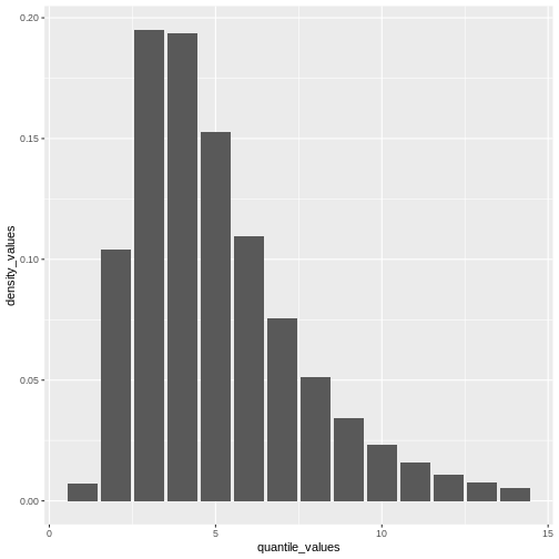
From a maximum value with quantile(), we can create a
sequence of quantile values as a numeric vector and calculate
density() values for each:
R
# create a discrete distribution visualisation
# from a maximum value from the distribution
quantile(covid_serialint_discrete, p = 0.99) %>%
  # generate quantile values
  # as a sequence for each natural number
  seq(1L, to = ., by = 1L) %>%
  # coerce numeric vector to data frame
  as_tibble_col(column_name = "quantile_values") %>%
  mutate(
    # calculate density values
    # for each quantile in the density function
    density_values =
      density(
        x = covid_serialint_discrete,
        at = quantile_values
      )
  ) %>%
  # create plot
  ggplot(
    aes(
      x = quantile_values,
      y = density_values
    )
  ) +
  geom_col()
Remember: In infections with pre-symptomatic transmission, serial intervals can have negative values (Nishiura et al., 2020). When we use the serial interval to approximate the generation time we need to make this distribution with positive values only!
Plug-in {epiparameter} to {EpiNow2}
Now we can plug everything into the EpiNow2::LogNormal()
function!
- the summary statistics
meanandsdof the distribution, - a maximum value
max, - the
distributionname.
When using EpiNow2::LogNormal() to define a log
normal distribution like the one in the
covid_serialint object we can specify the mean and sd as
parameters. Alternatively, to get the “natural” parameters for a log
normal distribution we can convert its summary statistics to
distribution parameters named meanlog and
sdlog. With {epiparameter} we can directly get
the distribution parameters using
epiparameter::get_parameters():
R
covid_serialint_parameters <-
  epiparameter::get_parameters(covid_serialint)
Then, we have:
R
serial_interval_covid <-
  EpiNow2::LogNormal(
    meanlog = covid_serialint_parameters["meanlog"],
    sdlog = covid_serialint_parameters["sdlog"],
    max = covid_serialint_discrete_max
  )

serial_interval_covid
OUTPUT
- lognormal distribution (max: 14):
  meanlog:
    1.4
  sdlog:
    0.57
Assuming a COVID-19 scenario, let’s use the first 60 days of the
example_confirmed data set from the EpiNow2
package as reported_cases and the recently created
serial_interval_covid object as inputs to estimate the
time-varying reproduction number using
EpiNow2::epinow().
R
epinow_estimates_cg <- epinow(
  # cases
  data = example_confirmed[1:60],
  # delays
  generation_time = generation_time_opts(serial_interval_covid)
)
OUTPUT
WARN [2024-06-18 17:33:18] epinow: There were 19 divergent transitions after warmup. See
https://mc-stan.org/misc/warnings.html#divergent-transitions-after-warmup
to find out why this is a problem and how to eliminate them. -
WARN [2024-06-18 17:33:18] epinow: Examine the pairs() plot to diagnose sampling problems
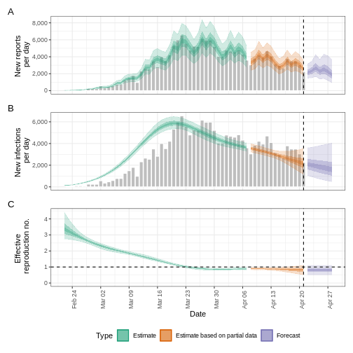
- R
base::plot(epinow_estimates_cg)
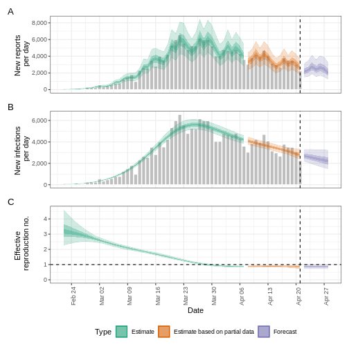
The plot() output includes the estimated cases by date
of infection, which are reconstructed from the reported cases and
delays.
Warning
Using the serial interval instead of the generation time is an alternative that can propagate bias in your estimates, even more so in diseases with reported pre-symptomatic transmission. (Chung Lau et al., 2021)
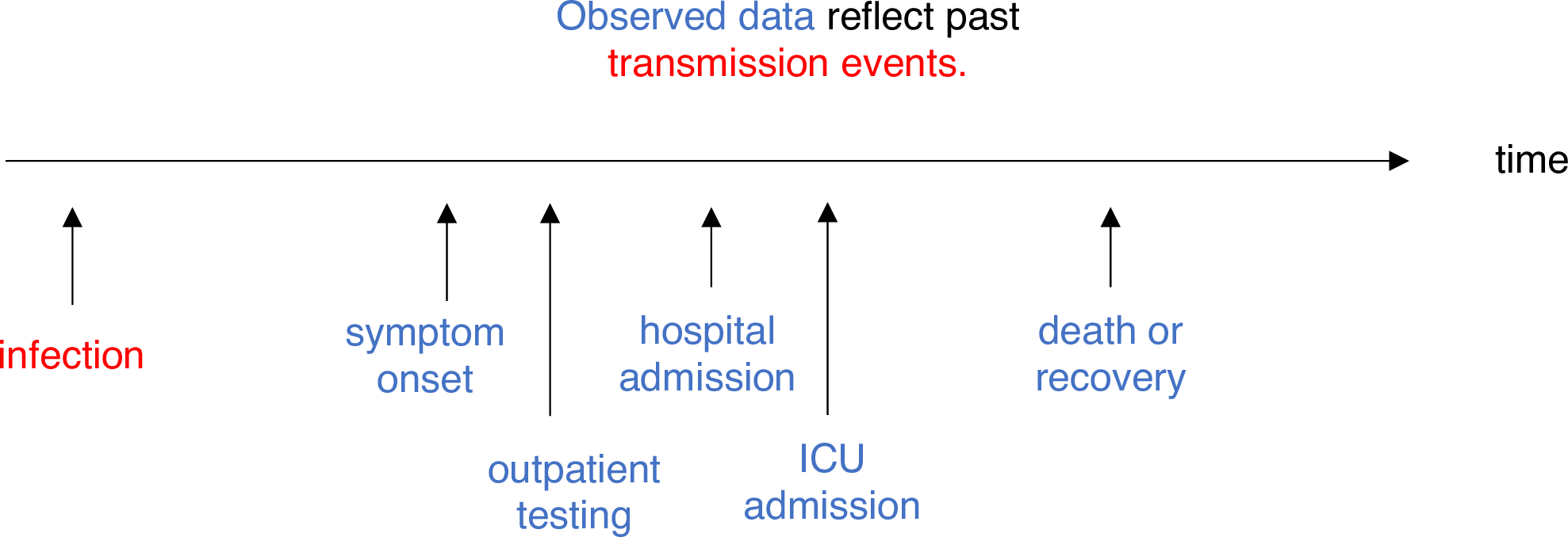
Adjusting for reporting delays
Estimating \(R_t\) requires data on the daily number of new infections. Due to lags in the development of detectable viral loads, symptom onset, seeking care, and reporting, these numbers are not readily available. All observations reflect transmission events from some time in the past. In other words, if \(d\) is the delay from infection to observation, then observations at time \(t\) inform \(R_{t−d}\), not \(R_t\). (Gostic et al., 2020)
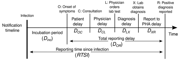
The delay distribution could be inferred jointly
with the underlying times of infection or estimated as the sum of the incubation period distribution and
the distribution of delays from symptom onset to observation from line
list data (reporting delay).
For EpiNow2, we can specify these two complementary delay
distributions in the delays argument.
Use an incubation period for COVID-19 to estimate Rt
Estimate the time-varying reproduction number for the first 60 days
of the example_confirmed data set from
EpiNow2. Access to an incubation period for COVID-19 from
{epiparameter} to use it as a reporting delay.
Use the last epinow() calculation using the
delays argument and the delay_opts() helper
function.
The delays argument and the delay_opts()
helper function are analogous to the generation_time
argument and the generation_time_opts() helper
function.
R
epinow_estimates <- epinow(
  # cases
  reported_cases = example_confirmed[1:60],
  # delays
  generation_time = generation_time_opts(covid_serial_interval),
  delays = delay_opts(covid_incubation_time)
)
R
# generation time ---------------------------------------------------------

# get covid serial interval
covid_serialint <-
  epiparameter::epidist_db(
    disease = "covid",
    epi_dist = "serial",
    author = "Nishiura",
    single_epidist = TRUE
  )

# adapt epidist to epinow2
covid_serialint_discrete_max <- covid_serialint %>%
  epiparameter::discretise() %>%
  quantile(p = 0.99)

covid_serialint_parameters <-
  epiparameter::get_parameters(covid_serialint)

covid_serial_interval <-
  EpiNow2::LogNormal(
    meanlog = covid_serialint_parameters["meanlog"],
    sdlog = covid_serialint_parameters["sdlog"],
    max = covid_serialint_discrete_max
  )

# incubation time ---------------------------------------------------------

# get covid incubation period
covid_incubation <- epiparameter::epidist_db(
  disease = "covid",
  epi_dist = "incubation",
  author = "Natalie",
  single_epidist = TRUE
)

# adapt epiparameter to epinow2
covid_incubation_discrete_max <- covid_incubation %>%
  epiparameter::discretise() %>%
  quantile(p = 0.99)

covid_incubation_parameters <-
  epiparameter::get_parameters(covid_incubation)

covid_incubation_time <-
  EpiNow2::LogNormal(
    meanlog = covid_incubation_parameters["meanlog"],
    sdlog = covid_incubation_parameters["sdlog"],
    max = covid_incubation_discrete_max
  )

# epinow ------------------------------------------------------------------

# run epinow
epinow_estimates_cgi <- epinow(
  # cases
  data = example_confirmed[1:60],
  # delays
  generation_time = generation_time_opts(covid_serial_interval),
  delays = delay_opts(covid_incubation_time)
)
OUTPUT
WARN [2024-06-18 17:35:46] epinow: There were 6 divergent transitions after warmup. See
https://mc-stan.org/misc/warnings.html#divergent-transitions-after-warmup
to find out why this is a problem and how to eliminate them. -
WARN [2024-06-18 17:35:46] epinow: Examine the pairs() plot to diagnose sampling problems
 -
R
base::plot(epinow_estimates_cgi)
Try to complement the delays argument with a reporting
delay like the reporting_delay_fixed object of the previous
episode.
How much has it changed?
After adding the incubation period, discuss:
- Does the trend of the model fit in the “Estimate” section change?
- Has the uncertainty changed?
- How would you explain or interpret any of these changes?
Compare all the EpiNow2 figures generated previously.
Challenges
A code completion tip
If we write the [] next to the object
covid_serialint_parameters[], within [] we can
use the Tab key ↹ for code
completion feature
This gives quick access to
covid_serialint_parameters["meanlog"] and
covid_serialint_parameters["sdlog"].
We invite you to try this out in code chunks and the R console!
Ebola’s effective reproduction number adjusted by reporting delays
Download and read the Ebola dataset:
- Estimate the effective reproduction number using EpiNow2
- Adjust the estimate by the available reporting delays in
{epiparameter} - Why did you choose that parameter?
To calculate the \(R_t\) using EpiNow2, we need:
- Aggregated incidence
data, with confirmed cases per day, and - The
generationtime distribution. - Optionally, reporting
delaysdistributions when available (e.g., incubation period).
To get delay distribution using {epiparameter} we can
use functions like:
epiparameter::epidist_db()epiparameter::parameter_tbl()discretise()quantile()
R
# read data
# e.g.: if path to file is data/raw-data/ebola_cases.csv then:
ebola_confirmed <-
  read_csv(here::here("data", "raw-data", "ebola_cases.csv"))

# list distributions
epiparameter::epidist_db(disease = "ebola") %>%
  epiparameter::parameter_tbl()
R
# generation time ---------------------------------------------------------

# subset one distribution for the generation time
ebola_serial <- epiparameter::epidist_db(
  disease = "ebola",
  epi_dist = "serial",
  single_epidist = TRUE
)

# adapt epiparameter to epinow2
ebola_serial_discrete <- epiparameter::discretise(ebola_serial)

serial_interval_ebola <-
  EpiNow2::Gamma(
    mean = ebola_serial$summary_stats$mean,
    sd = ebola_serial$summary_stats$sd,
    max = quantile(ebola_serial_discrete, p = 0.99)
  )

# incubation time ---------------------------------------------------------

# subset one distribution for delay of the incubation period
ebola_incubation <- epiparameter::epidist_db(
  disease = "ebola",
  epi_dist = "incubation",
  single_epidist = TRUE
)

# adapt epiparameter to epinow2
ebola_incubation_discrete <- epiparameter::discretise(ebola_incubation)

incubation_period_ebola <-
  EpiNow2::Gamma(
    mean = ebola_incubation$summary_stats$mean,
    sd = ebola_incubation$summary_stats$sd,
    max = quantile(ebola_serial_discrete, p = 0.99)
  )

# epinow ------------------------------------------------------------------

# run epinow
epinow_estimates_egi <- epinow(
  # cases
  data = ebola_confirmed,
  # delays
  generation_time = generation_time_opts(serial_interval_ebola),
  delays = delay_opts(incubation_period_ebola)
)
OUTPUT
WARN [2024-06-18 17:38:01] epinow: There were 7 divergent transitions after warmup. See
https://mc-stan.org/misc/warnings.html#divergent-transitions-after-warmup
to find out why this is a problem and how to eliminate them. -
WARN [2024-06-18 17:38:01] epinow: Examine the pairs() plot to diagnose sampling problems
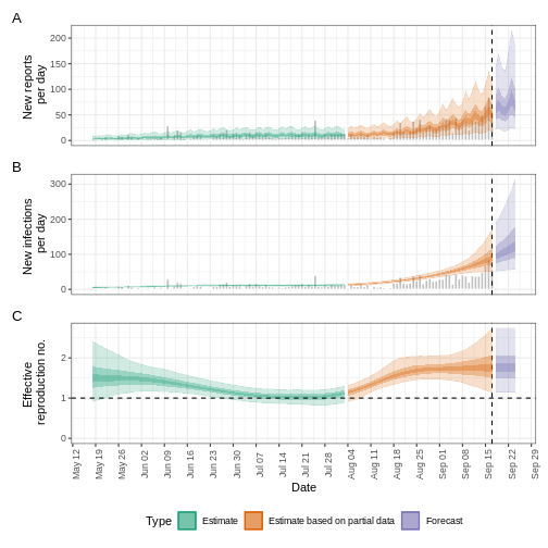
- R
plot(epinow_estimates_egi)
EpiNow2::NonParametric() accepts Probability Mass
Functions (PMF) from any distribution family. Read the reference guide
on Probability
distributions.
R
# What parameters are available for Influenza?
epiparameter::epidist_db(disease = "influenza") %>%
  epiparameter::parameter_tbl() %>%
  count(epi_distribution)
OUTPUT
# Parameter table:
# A data frame:    3 × 2
  epi_distribution      n
  <chr>             <int>
1 generation time       1
2 incubation period    15
3 serial interval       1
R
# generation time ---------------------------------------------------------

# Read the generation time
influenza_generation <-
  epiparameter::epidist_db(
    disease = "influenza",
    epi_dist = "generation"
  )

influenza_generation
OUTPUT
Disease: Influenza
Pathogen: Influenza-A-H1N1
Epi Distribution: generation time
Study: Lessler J, Reich N, Cummings D, New York City Department of Health and
Mental Hygiene Swine Influenza Investigation Team (2009). "Outbreak of
2009 Pandemic Influenza A (H1N1) at a New York City School." _The New
England Journal of Medicine_. doi:10.1056/NEJMoa0906089
<https://doi.org/10.1056/NEJMoa0906089>.
Distribution: weibull
Parameters:
  shape: 2.360
  scale: 3.180
R
# EpiNow2 currently accepts Gamma or LogNormal
# other can pass the PMF function

influenza_generation_discrete <-
  epiparameter::discretise(influenza_generation)

influenza_generation_max <-
  quantile(influenza_generation_discrete, p = 0.99)

influenza_generation_pmf <-
  density(
    influenza_generation_discrete,
    at = 1:influenza_generation_max
  )

influenza_generation_pmf
OUTPUT
[1] 0.06312336 0.22134988 0.29721220 0.23896828 0.12485164 0.04309454R
# EpiNow2::NonParametric() can also accept the PMF values
generation_time_influenza <-
  EpiNow2::NonParametric(
    pmf = influenza_generation_pmf
  )

# incubation period -------------------------------------------------------

# Read the incubation period
influenza_incubation <-
  epiparameter::epidist_db(
    disease = "influenza",
    epi_dist = "incubation",
    single_epidist = TRUE
  )

# Discretize incubation period
influenza_incubation_discrete <-
  epiparameter::discretise(influenza_incubation)

influenza_incubation_max <-
  quantile(influenza_incubation_discrete, p = 0.99)

influenza_incubation_pmf <-
  density(
    influenza_incubation_discrete,
    at = 1:influenza_incubation_max
  )

influenza_incubation_pmf
OUTPUT
[1] 0.05749151 0.16687705 0.22443092 0.21507632 0.16104546 0.09746609 0.04841928R
# EpiNow2::NonParametric() can also accept the PMF values
incubation_time_influenza <-
EpiNow2::NonParametric(
pmf = influenza_incubation_pmf
)
# epinow ------------------------------------------------------------------
# Read data
influenza_cleaned <-
outbreaks::influenza_england_1978_school %>%
select(date, confirm = in_bed)
# Run epinow()
epinow_estimates_igi <- epinow(
# cases
data = influenza_cleaned,
# delays
generation_time = generation_time_opts(generation_time_influenza),
delays = delay_opts(incubation_time_influenza)
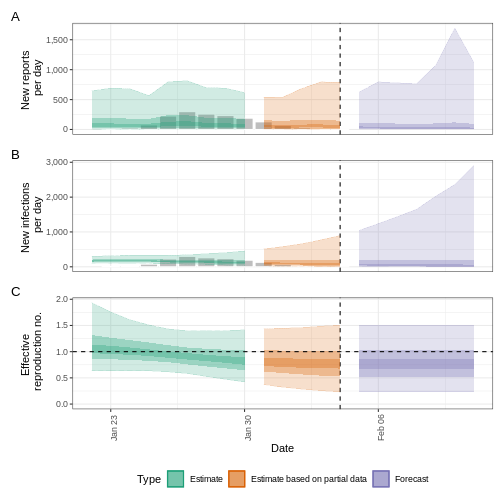
)
plot(epinow_estimates_igi)
Next steps
How to get distribution parameters from statistical distributions?
How to get the mean and standard deviation from a generation time
with only distribution parameters but no summary statistics
like mean or sd for
EpiNow2::Gamma() or EpiNow2::LogNormal()?
Look at the {epiparameter} vignette on parameter
extraction and conversion and its use
cases!
How to estimate delay distributions for Disease X?
Refer to this excellent tutorial on estimating the serial interval and incubation period of Disease X accounting for censoring using Bayesian inference with packages like rstan and coarseDataTools.
- Tutorial in English: https://rpubs.com/tracelac/diseaseX
- Tutorial en Español: https://epiverse-trace.github.io/epimodelac/EnfermedadX.html
Then, after you get your estimated values, you can
manually create your own<epidist> class objects with
epiparameter::epidist()! Take a look at its reference
guide on “Create an <epidist> object”!
Key Points
- Use distribution functions with
<epidist>objects to get summary statistics and informative parameters for public health interventions like the Window for contact tracing and Length of quarantine. - Use
discretise()to convert continuous to discrete delay distributions. - Use
{epiparameter}to get reporting delays required in transmissibility estimates.