Mpox Data cleaning and standardization pipeline
Last updated on 2026-07-14 | Edit this page
Introduction
In this document, we use the {cleanepi} package
to clean and standardize a messy mpox (formerly known as Monkeypox)
dataset obtained from the global.health platform. The dataset is
in a csv format available on this link.
We begin by importing the data into R and then utilize {cleanepi} functionalities to perform the following operations in a streamlined manner:
- Replace missing data with
NA. - Remove constant columns, empty rows, and columns.
- Detect and remove duplicate rows.
- Standardize the date columns by ensuring all date values follow the
format
YYYY-MM-DD(e.g.,2024-12-01for December 1st, 2024).
All these operations can be efficiently performed in a few lines as demonstrated in the following pipeline:
R
cleaned_data <-
  data.table::fread(
    "https://ivcjkmyexc.execute-api.eu-central-1.amazonaws.com/web/url?folder=&file_name=latest.csv") |>
  cleanepi::replace_missing_values(na_strings = "") |>
  cleanepi::remove_constants() |>
  cleanepi::standardize_dates(error_tolerance = 1) |>
  cleanepi::remove_duplicates()
In the sections below, we provide a detailed explanation of how these cleaning operations work.
Installing the required packages
We will need the following four packages:
-
data.table for fast import of large dataset. If you
have a smaller dataset you can use
readr::read_csv()orread.csv()instead. - cleanepi for data cleaning and standardization.
- wakefield for data visualization. For smaller datasets, you can use the visdat package.
- kableExtra for tabular visualization.
The below code chunk installs these packages (if not already installed).
R
# install the packages if not already done
# nolint start

if (!require("wakefield")) pak::pak("wakefield")
if (!require("cleanepi")) pak::pak("cleanepi")
if (!require("kableExtra")) pak::pak("kableExtra")
if (!require("data.table")) pak::pak("data.table")

# nolint end
# load the libraries
library(wakefield)
library(cleanepi)
library(kableExtra)
library(data.table)
Data download
The data file is quite large (\(\sim
17\) MB) and may fail to download using read.csv()
due to time limits. As such, we recommend to import the data using the
data.table::fread() function or download it on your
computer.
We load the dataset using the data.table::fread()
function and visualize it with both View() and
wakefield::table_heat() functions to understand the
distribution of missing values within the dataset.
R
# import the data
data_in <- data.table::fread(
  "https://ivcjkmyexc.execute-api.eu-central-1.amazonaws.com/web/url?folder=&file_name=latest.csv"
)

# Visualise the distribution of the different types as well as missing data
# across the dataset
wakefield::table_heat(data_in, palette = "Set3", flip = TRUE, print = TRUE)
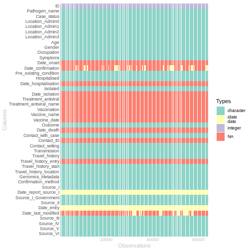
As show in the above figure, the dataset contains 45 columns and 64215 rows. Approximately 81.04% of the values are missing, of which around 53.08% is represented by empty strings.
Use NA for missing data
Missing values appear as empty strings in the data. To ensure
consistency with the R language, we will standardize these missing
values as NA using the
replace_missing_values() function from
cleanepi.
R
# Replace empty characters ("") with NA
data_in <- data_in |>
  cleanepi::replace_missing_values(na_strings = "")
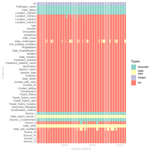
After replacing the empty characters with NA, the
dataset is now composed of 81.04% missing values. The new distribution
of missing values is shown in the below figure.
R
# Visualise the new distribution of the different data types as well as missing
# data across the dataset
wakefield::table_heat(data_in, palette = "Set3", flip = TRUE, print = TRUE)
Scan through character columns
To determine which potential data cleaning operations could be
applied to this dataset, we can examine all the content of the character
columns by assessing the proportion of the various data types. This can
be accomplished using the scan_data() function from the
cleanepi package.
R
# Scan with cleanepi
scan_result <- cleanepi::scan_data(data_in)
In the below code chunk, we make sure to color in red any row where
there are multiple data types found by the scan_data()
function.
R
# detect rows with multiple data types
df <- scan_result |>
  dplyr::mutate(
    highlight = ((numeric > 0) & (date > 0)) |
      ((numeric > 0) & (character > 0)) |
      ((numeric > 0) & (logical > 0)) |
      ((date > 0) & (character > 0)) |
      ((date > 0) & (logical > 0)) |
      ((character > 0) & (logical > 0))
  )
highlight_rows <- which(df$highlight)

scan_result |>
  kableExtra::kable() |>
  kableExtra::kable_paper("striped", font_size = 14, full_width = TRUE) |>
  kableExtra::scroll_box(height = "200px", width = "100%",
                         box_css = "border: 1px solid #ddd; padding: 5px;",
                         extra_css = NULL,
                         fixed_thead = TRUE) |>
  kableExtra::row_spec(highlight_rows, bold = TRUE,
                       background = "red", color = "white")
| Field_names | missing | numeric | date | character | logical |
|---|---|---|---|---|---|
| Pathogen_name | 0.0000 | 0 | 0 | 1 | 0 |
| Case_status | 0.0000 | 0 | 0 | 1 | 0 |
| Location_Admin0 | 0.0000 | 0 | 0 | 1 | 0 |
| Location_Admin1 | 40.0319 | 0 | 0 | 1 | 0 |
| Location_Admin2 | 1426.0000 | 0 | 0 | 1 | 0 |
| Location_Admin3 | 32106.5000 | 0 | 0 | 1 | 0 |
| Age | 1051.7049 | 0 | 0 | 1 | 0 |
| Gender | 1087.3898 | 0 | 0 | 1 | 0 |
| Occupation | 5350.2500 | 0 | 0 | 1 | 0 |
| Symptoms | 1604.3750 | 0 | 0 | 1 | 0 |
| Pre_existing_condition | 4585.7857 | 0 | 0 | 1 | 0 |
| Hospitalised | 1734.5405 | 0 | 0 | 1 | 0 |
| Isolated | 2674.6250 | 0 | 0 | 1 | 0 |
| Outcome | 791.7778 | 0 | 0 | 1 | 0 |
| Contact_with_case | 4012.4375 | 0 | 0 | 1 | 0 |
| Contact_setting | 9172.5714 | 0 | 0 | 1 | 0 |
| Transmission | 32106.5000 | 0 | 0 | 1 | 0 |
| Travel_history | 1492.3721 | 0 | 0 | 1 | 0 |
| Travel_history_start | 9172.5714 | 0 | 1 | 0 | 0 |
| Travel_history_location | 2790.9565 | 0 | 0 | 1 | 0 |
| Genomics_Metadata | 3209.7500 | 0 | 0 | 1 | 0 |
| Confirmation_method | 4585.7857 | 0 | 0 | 1 | 0 |
| Source_I | 0.0000 | 0 | 0 | 1 | 0 |
| Source_I_Government | 0.0001 | 0 | 0 | 1 | 0 |
| Source_II | 13.1912 | 0 | 0 | 1 | 0 |
| Source_III | 188.4248 | 0 | 0 | 1 | 0 |
| Source_IV | 227.5231 | 0 | 0 | 1 | 0 |
| Source_V | 1233.9038 | 0 | 0 | 1 | 0 |
| Source_VI | 8025.8750 | 0 | 0 | 1 | 0 |
In the table above, each row represents a column from the original dataset, while the columns indicate different data types. If a row has a non-zero percentage in more than one data type (excluding missing values), its corresponding column in the original dataset needs to be standardized.
Remove constant columns
The dataset may contain constant columns (i.e. columns with the same
value across all rows) and empty rows and columns (i.e. rows or columns
with only NA values). To remove these non-informative rows
and columns, we use the remove_constants() function from
the cleanepi package.
R
# Remove constant columns, empty rows and columns
data_in <- data_in |>
  cleanepi::remove_constants()
This resulted in the removal of 11 columns — 5 empty columns and 6 constant columns — while no empty rows were removed, as shown in the table below.
R
# display the set of constant data
constant_data <- cleanepi::print_report(data_in, "constant_data")
constant_data |>
  kableExtra::kbl() |>
  kableExtra::kable_paper("striped", font_size = 14, full_width = TRUE) |>
  kableExtra::scroll_box(height = "200px", width = "100%",
                         box_css = "border: 1px solid #ddd; padding: 5px; ",
                         extra_css = NULL,
                         fixed_thead = TRUE)
| iteration | empty_columns | empty_rows | constant_columns |
|---|---|---|---|
| 1 | Treatment_antiviral, Treatment_antiviral_name, Vaccination, Vaccine_name, Vaccine_date | NA | Pathogen_name, Pre_existing_condition, Isolated, Date_isolation, Contact_with_case, Transmission |
Remove duplicates
We can detect and remove duplicates using the
remove_duplicates() function from the
cleanepi package. In this case, we do not specify any
target column, i.e., we look for duplicates across all columns.
R
data_in <- data_in |>
  cleanepi::remove_duplicates()
OUTPUT
ℹ No duplicates were found.Fortunately (or unfortunately!) there are no duplicate entries in this dataset.
Standardise dates
Some character columns seem to contain actual Date values. We will
apply the standardize_dates() function from the
cleanepi package to ensure all date columns are in
ISO8601 format. First, we’ll identify the potential Date columns from
the results of the scan_data() function, and then use those
columns for standardization.
R
# Identify potential Date columns from the scanning results. Columns with
# %date > 0 are likely to be of type Date
potential_dates <- scan_result |>
  dplyr::filter(date > 0)
target_columns <- potential_dates$Field_names

# Standardise the selected columns
data_in <- data_in |>
  cleanepi::standardize_dates(
    target_columns = target_columns,
    error_tolerance = 1
  )
OUTPUT
! Detected no values that comply with multiple formats and no values that are
  outside of the specified time frame.
ℹ Enter `print_report(data = dat, "date_standardization")` to access them,
  where "dat" is the object used to store the output from this operation.
Removing columns with excessive NA Values
After applying the above mentioned rudimentary cleaning operations,
the dataset still contains several columns with a high proportion of
NA values. These columns provide limited analytical value,
and thus less informative.
To remove such columns from the dataset and exclude them from further
downstream analysis, we can use the remove_constant()
function from cleanepi, setting the cutoff
parameter to an appropriate value.
For example, the below code chunk could be used to exclude columns
where more than 90% of the values are
NA.
R
df <- data_in |>
  cleanepi::remove_constants(cutoff = 0.9)

# Visualise the new distribution of missing data across the dataset
wakefield::table_heat(df, palette = "Set3", flip = TRUE, print = TRUE)
Conclusion
Data cleaning is an essential task for robust downstream statistical analysis. However, it can be tedious and time-consuming. By leveraging the efficient functionalities of cleanepi, users can clean and standardize their input datasets quickly and effectively, using minimal and concise code.