Getting started with epidemic scenario modelling components

This initial vignette shows to get started with using the epidemics package.

Further vignettes include guidance on “Modelling the implementation of vaccination regimes”, as well as on“Modelling non-pharmaceutical interventions (NPIs) to reduce social contacts” and “Modelling multiple overlapping NPIs”.

There is also guidance available on specific models in the model library, such as the Vacamole model developed by RIVM, the Dutch Institute for Public Health.

Code

library(epidemics)
library(dplyr)
#> 
#> Attaching package: 'dplyr'
#> The following objects are masked from 'package:stats':
#> 
#>     filter, lag
#> The following objects are masked from 'package:base':
#> 
#>     intersect, setdiff, setequal, union
library(ggplot2)

Prepare population and initial conditions

Prepare population and contact data.

Note on social contacts data

Note that the social contacts matrices provided by the socialmixr[https://CRAN.R-project.org/package=socialmixr] package follow a format wherein the matrix \(M_{ij}\) represents contacts from group \(i\) to group \(j\).

However, epidemic models traditionally adopt the notation that \(M_{ij}\) defines contacts to \(i\) from \(j\) (Wallinga, Teunis, and Kretzschmar 2006).

\(q M_{ij} / n_i\) then defines the probability of infection, where \(q\) is a scaling factor dependent on \(R_0\) (or another measure of infection transmissibility), and \(n_i\) is the population proportion of group \(i\). The ODEs in epidemics also follow this convention.

For consistency with this notation, social contact matrices from socialmixr need to be transposed (using t()) before they are used with epidemics.

Code

# load contact and population data from socialmixr::polymod
polymod <- socialmixr::polymod
contact_data <- socialmixr::contact_matrix(
  polymod,
  countries = "United Kingdom",
  age.limits = c(0, 20, 40),
  symmetric = TRUE
)
#> Removing participants that have contacts without age information. To change this behaviour, set the 'missing.contact.age' option

# prepare contact matrix
contact_matrix <- t(contact_data$matrix)

# prepare the demography vector
demography_vector <- contact_data$demography$population
names(demography_vector) <- rownames(contact_matrix)

# view contact matrix and demography
contact_matrix
#>                  
#> contact.age.group     [,1]     [,2]     [,3]
#>           [0,20)  7.883663 2.794154 1.565665
#>           [20,40) 3.120220 4.854839 2.624868
#>           40+     3.063895 4.599893 5.005571

demography_vector
#>   [0,20)  [20,40)      40+ 
#> 14799290 16526302 28961159

Prepare initial conditions for each age group.

Code

# initial conditions
initial_i <- 1e-6
initial_conditions <- c(
  S = 1 - initial_i, E = 0, I = initial_i, R = 0, V = 0
)

# build for all age groups
initial_conditions <- rbind(
  initial_conditions,
  initial_conditions,
  initial_conditions
)

# assign rownames for clarity
rownames(initial_conditions) <- rownames(contact_matrix)

# view initial conditions
initial_conditions
#>                S E     I R V
#> [0,20)  0.999999 0 1e-06 0 0
#> [20,40) 0.999999 0 1e-06 0 0
#> 40+     0.999999 0 1e-06 0 0

Prepare a population as a population class object.

Code

uk_population <- population(
  name = "UK",
  contact_matrix = contact_matrix,
  demography_vector = demography_vector,
  initial_conditions = initial_conditions
)

uk_population
#> <population> object
#> 
#>  Population name: 
#> "UK"
#> 
#>  Demography 
#> [0,20): 14,799,290 (20%)
#> [20,40): 16,526,302 (30%)
#> 40+: 28,961,159 (50%)
#> 
#>  Contact matrix 
#>                  
#> contact.age.group   [0,20)  [20,40)      40+
#>           [0,20)  7.883663 2.794154 1.565665
#>           [20,40) 3.120220 4.854839 2.624868
#>           40+     3.063895 4.599893 5.005571

Run epidemic model

Code

# run an epidemic model using `epidemic`
output <- model_default(
  population = uk_population,
  time_end = 600, increment = 1.0
)

Prepare data and visualise infections

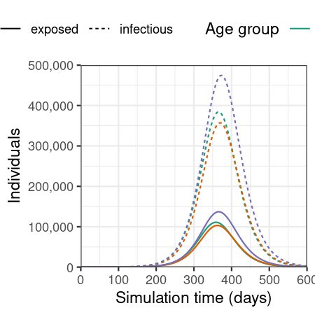
Plot epidemic over time, showing only the number of individuals in the exposed and infected compartments.

Code

# plot figure of epidemic curve
filter(output, compartment %in% c("exposed", "infectious")) %>%
  ggplot(
    aes(
      x = time,
      y = value,
      col = demography_group,
      linetype = compartment
    )
  ) +
  geom_line() +
  scale_y_continuous(
    labels = scales::comma
  ) +
  scale_colour_brewer(
    palette = "Dark2",
    name = "Age group"
  ) +
  expand_limits(
    y = c(0, 500e3)
  ) +
  coord_cartesian(
    expand = FALSE
  ) +
  theme_bw() +
  theme(
    legend.position = "top"
  ) +
  labs(
    x = "Simulation time (days)",
    linetype = "Compartment",
    y = "Individuals"
  )

References

Wallinga, Jacco, Peter Teunis, and Mirjam Kretzschmar. 2006. “Using Data on Social Contacts to Estimate Age-Specific Transmission Parameters for Respiratory-Spread Infectious Agents.” American Journal of Epidemiology 164 (10): 936–44. https://doi.org/10.1093/aje/kwj317.