Modelling a diphtheria outbreak in a humanitarian camp setting

New to epidemics? It may help to read the “Get started” vignette first!

This vignette shows how to model an outbreak of diphtheria (or a similar acute directly-transmitted infectious disease) within the setting of a humanitarian aid camp, where the camp population may fluctuate due to external factors, including influxes from crisis affected areas or evacuations to other camps or areas. In such situations, implementing large-scale public health measures such contact tracing and quarantine, or introducing reactive mass vaccination may be challenging.

The vignette on modelling a vaccination campaign shows how to model the introduction of a mass vaccination campaign for a fixed, stable population.

epidemics provides a simple SEIHR compartmental model based on Finger et al. (2019), in which it is possible to vary the population of each demographic group throughout the model’s simulation time and explore the resulting epidemic dynamics. This baseline model only tracks infections by demographic groups, and does not include variation in contacts between demographic groups (e.g. by age or occupation), as contacts are likely to be less clearly stratified in a camp setting. The baseline model also does not allow interventions that target social contacts (such as social distancing or quarantine), and does not include a ‘vaccinated’ compartment. It is therefore suited to analysis of a rapidly spreading infection prior to the introduction of any reactive vaccine campaign.

However, the model does allow for seasonality in model parameters and interventions on model parameters. Similarly, the model allows for a proportion of the initial camp population to be considered vaccinated and thus immune from infection.

Code

library(epidemics)
library(dplyr)
library(ggplot2)

Modelling an outbreak with pre-existing immunity

We create a population object corresponding to the Kutupalong camp in Cox’s Bazar, Bangladesh in 2017-18, rounded to the nearest 100, as described in Additional file 1 provided with Finger et al. (2019). This population has three age groups, < 5 years, 5 – 14 years, \(\geq\) 15 years. We assume that only one individual is infectious in each age group.

Code

# three age groups with five compartments SEIHR
n_age_groups <- 3
demography_vector <- c(83000, 108200, 224600)
initial_conditions <- matrix(0, nrow = n_age_groups, ncol = 5)

# 1 individual in each group is infectious
initial_conditions[, 1] <- demography_vector - 1
initial_conditions[, 3] <- rep(1, n_age_groups)

# camp social contact rates are assumed to be uniform within and between
# age groups
camp_pop <- population(
  contact_matrix = matrix(1, nrow = n_age_groups, ncol = n_age_groups),
  demography_vector = demography_vector,
  initial_conditions = initial_conditions / demography_vector
)

camp_pop
#> 
#>  Population name: 
#>  Demography 
#> Dem. grp. 1: 83,000 (20%)
#> Dem. grp. 2: 108,200 (30%)
#> Dem. grp. 3: 224,600 (50%)
#> 
#>  Contact matrix 
#>              Dem. grp. 1: Dem. grp. 2: Dem. grp. 3:
#> Dem. grp. 1:            1            1            1
#> Dem. grp. 2:            1            1            1
#> Dem. grp. 3:            1            1            1

We assume, following Finger et al. (2019), that 20% of the 5 – 14 year-olds were vaccinated against (and immune to) diphtheria prior to the start of the outbreak, but that coverage is much lower among other age groups.

Code

# 20% of 5-14 year-olds are vaccinated
prop_vaccinated <- c(0.05, 0.2, 0.05)

We run the model with its default parameters, assuming that:

• diphtheria has an \(R_0\) of 4.0 and a mean infectious period of 4.5 days, giving a transmission rate (\(\beta\)) of about 0.889;
• diphtheria has a pre-infectious or incubation period of 3 days, giving an infectiousness rate (\(\sigma\)) of about 0.33; and
• the recovery rate of diphtheria is about 0.33.

We also make several assumptions regarding clinical progression and reporting. Specifically: case reporting (that about 3% of infections are reported as cases), the proportion of reported cases needing hospitalisation (1%), the time taken by cases needing hospitalisation to seek and be admitted to hospital (5 days, giving a daily hospitalisation rate of 0.2 among cases), and time spent in hospital (5 days, giving a daily hospitalisation recovery rate of 0.2).

Finally, we assume there are no interventions or seasonal effects that affect the dynamics of transmission during the outbreak. We then run the model and plot the outcomes.

Code

data <- model_diphtheria(
  population = camp_pop,
  prop_vaccinated = prop_vaccinated
)

Code

filter(data, compartment == "infectious") %>%
  ggplot() +
  geom_line(
    aes(time, value, colour = demography_group)
  ) +
  scale_y_continuous(
    labels = scales::comma
  ) +
  scale_colour_brewer(
    palette = "Dark2",
    name = "Age group",
    labels = c("<5", "5-15", ">15")
  ) +
  expand_limits(
    x = c(0, 101)
  ) +
  theme_bw() +
  theme(
    legend.position = "top"
  ) +
  labs(
    x = "Simulation time (days)",
    y = "Individuals infectious"
  )

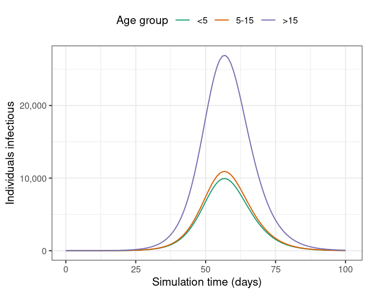
Figure 1: Model results from a single run showing the number of individuals infectious with diphtheria over 100 days of the outbreak.

Modelling an outbreak with changing population sizes

We now model the same outbreak, but an increase in susceptible individuals towards the end of the outbreak, to illustrate the effect that an influx of non-immune individuals could could have on outbreak dynamics. In this example, we do not assume any prior immunity among new arrivals into the population.

We prepare a population change schedule as a named list giving the times of each change, and the corresponding changes to each demographic group.

Note that the model assumes that these changes apply only to the susceptible compartment, as we assume that the wider population entering the camp is not yet affected by diphtheria (i.e. no infected or recovered arrival), and that already infected or hospitalised individuals do not leave the camp.

Code

# susceptibles increase by about 12%, 92%, and 89% of initial sizes
pop_change <- list(
  time = 70,
  values = list(
    c(1e4, 1e5, 2e5)
  )
)

Here, the population size of the camp increases by about 75% overall, which is similar to reported values in the Kutupalong camp scenario (Finger et al. 2019).

Code

data <- model_diphtheria(
  population = camp_pop,
  population_change = pop_change
)

# summarise population change in susceptibles
data_pop_size <- filter(data, compartment == "susceptible") %>%
  group_by(time) %>%
  summarise(
    total_susceptibles = sum(value)
  )

Code

ggplot() +
  geom_area(
    data = data_pop_size,
    aes(time, total_susceptibles / 10),
    fill = "steelblue", alpha = 0.5
  ) +
  geom_line(
    data = filter(data, compartment == "infectious"),
    aes(time, value, colour = demography_group)
  ) +
  geom_vline(
    xintercept = pop_change$time,
    colour = "red",
    linetype = "dashed",
    linewidth = 0.2
  ) +
  annotate(
    geom = "text",
    x = pop_change$time,
    y = 20e3,
    label = "Population increase",
    angle = 90,
    vjust = "inward",
    colour = "red"
  ) +
  scale_y_continuous(
    labels = scales::comma,
    sec.axis = dup_axis(
      trans = function(x) x * 10,
      name = "Individuals susceptible"
    )
  ) +
  scale_colour_brewer(
    palette = "Dark2",
    name = "Age group (individuals infectious)",
    labels = c("<5", "5-15", ">15")
  ) +
  expand_limits(
    x = c(0, 101)
  ) +
  theme_bw() +
  theme(
    legend.position = "top"
  ) +
  labs(
    x = "Simulation time (days)",
    y = "Individuals infectious"
  )

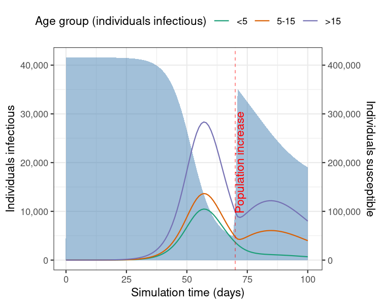
Figure 2: Model results from a single run showing the number of individuals infectious with diphtheria over 100 days of the outbreak, with an increase in the camp population size. Shaded blue region shows the number of individuals susceptible to infection (right-hand side Y axis).

This example shows how an increase in the number of susceptibles in the population can lead to a rise in the transmission potential of the infection and therefore extend the duration of an outbreak.

References

Finger, Flavio, Sebastian Funk, Kate White, M. Ruby Siddiqui, W. John Edmunds, and Adam J. Kucharski. 2019. “Real-Time Analysis of the Diphtheria Outbreak in Forcibly Displaced Myanmar Nationals in Bangladesh.” BMC Medicine 17 (March): 58. https://doi.org/10.1186/s12916-019-1288-7.