Modelling responses to a stochastic Ebola virus epidemic

New to epidemics? It may help to read the “Get started” vignette first!

This vignette shows how to model an epidemic in which stochasticity is expected to play an important role. This is often the case with outbreaks of infections such as Ebola virus disease (EVD, or simply, ebola).

epidemics includes a discrete time, stochastic compartmental model of ebola based on a consensus model presented in Li et al. (2019), with six compartments — susceptible, exposed, infectious, hospitalised, funeral, and removed. The transitions between compartments are based on an Erlang model developed by Getz and Dougherty (2018) for the 2014 West African EVD outbreak, with the code adapted from Epirecipes.

The model allows easily running multiple replicates, accepts infection parameter vectors to help model parameter uncertainty, and can accept lists of intervention sets to model response scenarios.

Code

# some initial setup to load necessary packages
library(epidemics)
library(dplyr)
library(purrr)
library(tidyr)
library(withr)
library(ggplot2)

Prepare population and initial conditions

Prepare population data — for this model, we only need the total population size and the initial conditions.

We can create a <population> object with dummy values for the contact matrix, and assign the total size to the demography vector.

We prepare a population with a total size of 14 million, corresponding to the population of Guinea, a West African country where the 2014 Ebola virus epidemic originated.

We assume that 1 person is initially infected and infectious, and 10 other people have been exposed and is yet to become infectious.

Code

population_size <- 14e6

# prepare initial conditions as proportions
initial_conditions <- c(
  S = population_size - 11, E = 10, I = 1, H = 0, F = 0, R = 0
) / population_size

Code

# prepare a <population> object
guinea_population <- population(
  name = "Guinea",
  contact_matrix = matrix(1), # note dummy value
  demography_vector = 14e6, # 14 million, no age groups
  initial_conditions = matrix(
    initial_conditions,
    nrow = 1
  )
)

guinea_population
#> 
#>  Population name: 
#>  Demography 
#> Dem. grp. 1: 14,000,000 (100%)
#> 
#>  Contact matrix 
#>              Dem. grp. 1:
#> Dem. grp. 1:            1

Prepare model parameters

We use the default model parameters, beginning with an \(R_0\) taken from the value estimated for ebola in Guinea (Althaus 2014). We assume that ebola has a mean infectious period of 12 days, and that the time between exposure and symptom onset — the pre-infectious period — is 5 days.

Together, these give the following values:

• Transmission rate (\(\beta\)): 0.125,

• Infectiousness rate (\(\gamma^E\) in Getz and Dougherty (2018)): 0.4,

• Removal rate (\(\gamma^I\) in Getz and Dougherty (2018)): 0.1667

This model does not yet have an explicit “deaths” compartment, but rather, the “removed” compartment holds all individuals who have recovered and who have died and been buried safely. Functionally, they are similar as they are not part of the model dynamics.

We assume that only 10% of infectious individuals are hospitalised, and that hospitalisation achieves a modest 30% reduction in transmission between hospitalised individuals and those still susceptible.

We assume also that any deaths in hospital lead to ebola-safe funerals, such that no further infections result from them.

We assume that infectious individuals who are not hospitalised die in the community, and that their funerals are potentially not ebola-safe. We assume that the transmission rate of ebola at funerals is 50% of the baseline transmission rate. This can also be interpreted as the proportion of funerals that are ebola-safe.

Run epidemic model

We run the model using the function model_ebola().

The model is run for 100 days (the default), with data reported on each day. This is an appropriate period over which to obtain initial predictions for the outbreak, and after which response efforts such as non-pharmaceutical interventions and vaccination campaigns are likely to be launched to bring the outbreak under control.

The function automatically runs 100 replicates (stochastic realisations) as a default, and this can be changed using the replicates argument.

Code

# run with a pre-set seed for consisten results
# run the epidemic model using `epidemic`
# we call the model "ebola" from the library
data <- withr::with_seed(
  1,
  model_ebola(
    population = guinea_population
  )
)

# view the head of the output
head(data)
#>     time demography_group  compartment    value replicate
#>    <int>           <char>       <char>    <num>     <int>
#> 1:     0     demo_group_1  susceptible 13999989         1
#> 2:     0     demo_group_1      exposed       10         1
#> 3:     0     demo_group_1   infectious        1         1
#> 4:     0     demo_group_1 hospitalised        0         1
#> 5:     0     demo_group_1      funeral        0         1
#> 6:     0     demo_group_1      removed        0         1

Prepare data and visualise infections

We plot the size of the ebola epidemic over time; the epidemic size is taken to be the number of individuals considered ‘removed’.

Code

# plot figure of epidemic curve
filter(data, compartment == "removed") %>%
  ggplot(
    aes(
      x = time, y = value
    )
  ) +
  geom_line(aes(group = replicate), linewidth = 0.2, colour = "grey") +
  stat_summary(
    fun.min = function(x) quantile(x, 0.025),
    fun.max = function(x) quantile(x, 0.975),
    geom = "ribbon", fill = "red", alpha = 0.2
  ) +
  stat_summary(geom = "line") +
  scale_y_continuous(
    labels = scales::comma
  ) +
  expand_limits(
    x = c(0, 101),
    y = c(-10, NA)
  ) +
  coord_cartesian(expand = FALSE) +
  theme_bw() +
  theme(
    legend.position = "top"
  ) +
  labs(
    x = "Simulation time (days)",
    y = "Outbreak size"
  )

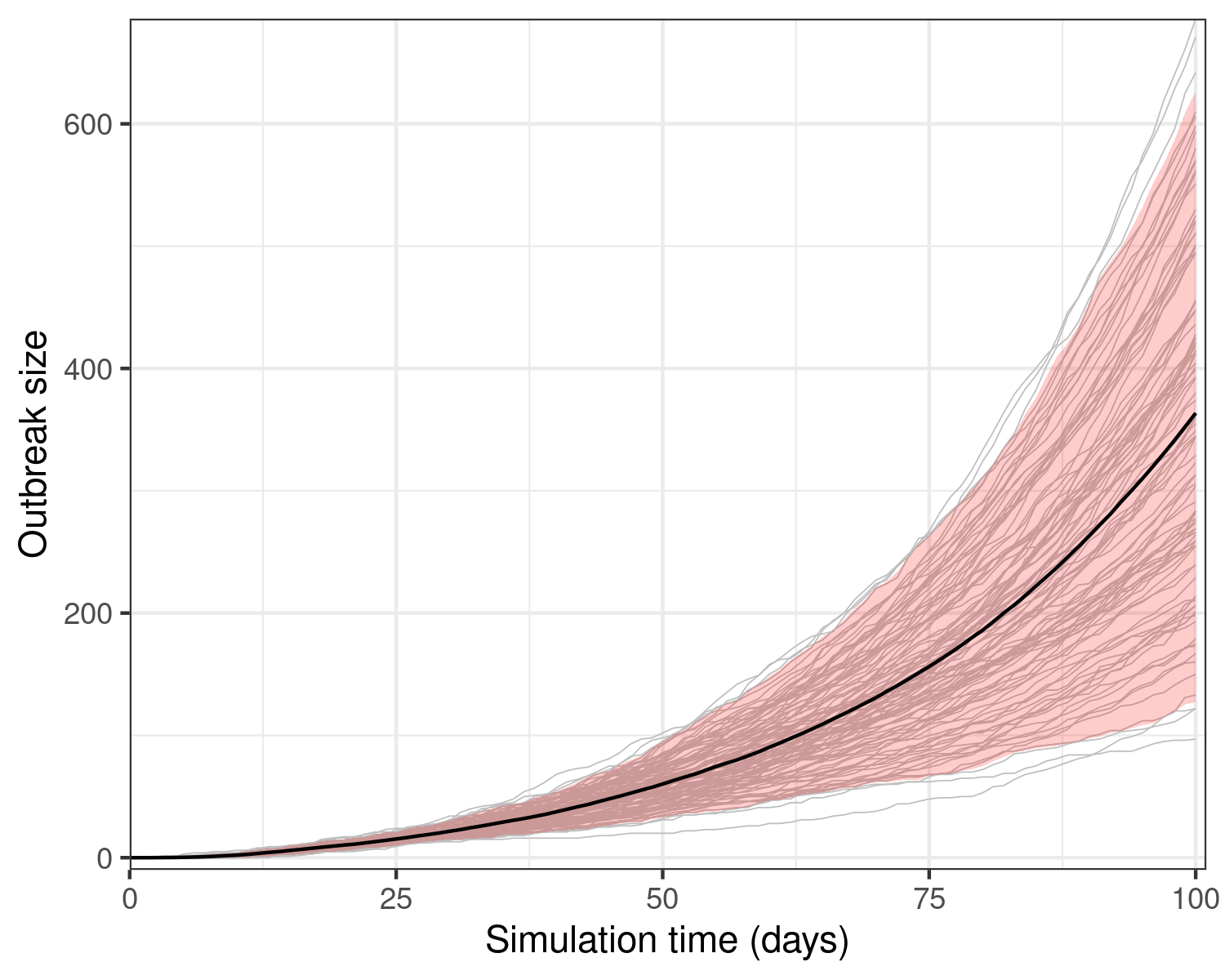
Figure 1: Model results from a single run showing the epidemic size over 100 days of the outbreak. The model assumes that 1 initially infectious person has exposed 10 others. Grey lines show 100 stochastic realisations or model replicates.

We observe that model stochasticity leads to wide variation in model outcomes within the first 100 days: some outbreaks may be much more severe than the mean outbreak. Note how in nearly all replicates, the epidemic size is increasing at near exponential rates.

We can find the size of each replicate using the epidemic_size() function on the original simulation data. Note that the final size here refers to the final size after 100 days, which is the duration of our simulation.

Code

# apply the function over each replicate
data_final_size <- nest(data, .by = "replicate") %>%
  mutate(
    final_size = map_dbl(data, epidemic_size)
  )

# get range of final sizes
range(data_final_size$final_size)
#> [1]  97 686

Looking to model parameter uncertainty? The vignette on modelling parameter uncertainty has helpful information that is also applicable to the Ebola model.

Applying interventions that reduce transmission

Interventions that affect model parameters (called rate interventions) can be simulated for an Ebola outbreak in the same way as for other models; creating and passing rate interventions is covered in the vignette on modelling rate interventions.

Note that the model does not include demographic variation in contacts, as EVD spreads primarily among contacts caring for infected individuals, making age or demographic structure less important. Thus this model allows interventions on model rates only (as there are no demographic groups for contacts interventions).

Here, we compare the effect of an intervention that begins 15 days into the outbreak, and reduces transmission by 20%, against the counterfactual, baseline scenario of no specific outbreak response. We simulate 100 days as in the previous examples.

Code

# create an intervention on the transmission rate
reduce_transmission <- intervention(
  type = "rate",
  time_begin = 15, time_end = 100, reduction = 0.2
)

# create a list of intervention scenarios
intervention_scenarios <- list(
  baseline = NULL,
  response = list(
    transmission_rate = reduce_transmission
  )
)

Code

# run the epidemic model and save data as the baseline, using a fixed seed
data_scenarios <- withr::with_seed(
  1,
  model_ebola(
    population = guinea_population,
    intervention = intervention_scenarios
  )
)

# assign scenario names
data_scenarios$scenario <- c("baseline", "response")

# unnest the data, preserving scenario identifiers
data_scenarios <- select(data_scenarios, data, scenario) %>%
  unnest(data)

Code

filter(data_scenarios, compartment == "removed") %>%
  ggplot(aes(time, value, colour = scenario)) +
  geom_vline(
    xintercept = 15,
    linetype = "dotted"
  ) +
  geom_line(
    aes(group = interaction(scenario, replicate)),
    linewidth = 0.2, alpha = 0.5
  ) +
  stat_summary(
    geom = "ribbon",
    fun.min = function(x) quantile(x, 0.025),
    fun.max = function(x) quantile(x, 0.975),
    alpha = 0.3, colour = NA,
    aes(fill = scenario)
  ) +
  stat_summary(
    geom = "line", linewidth = 1
  ) +
  scale_colour_brewer(
    palette = "Dark2",
    name = "Scenario",
    labels = c("Baseline", "Intervention")
  ) +
  scale_fill_brewer(
    palette = "Dark2",
    name = "Scenario",
    labels = c("Baseline", "Intervention")
  ) +
  theme_bw() +
  theme(
    legend.position = "top"
  ) +
  labs(
    x = "Days",
    y = "Outbreak size"
  )

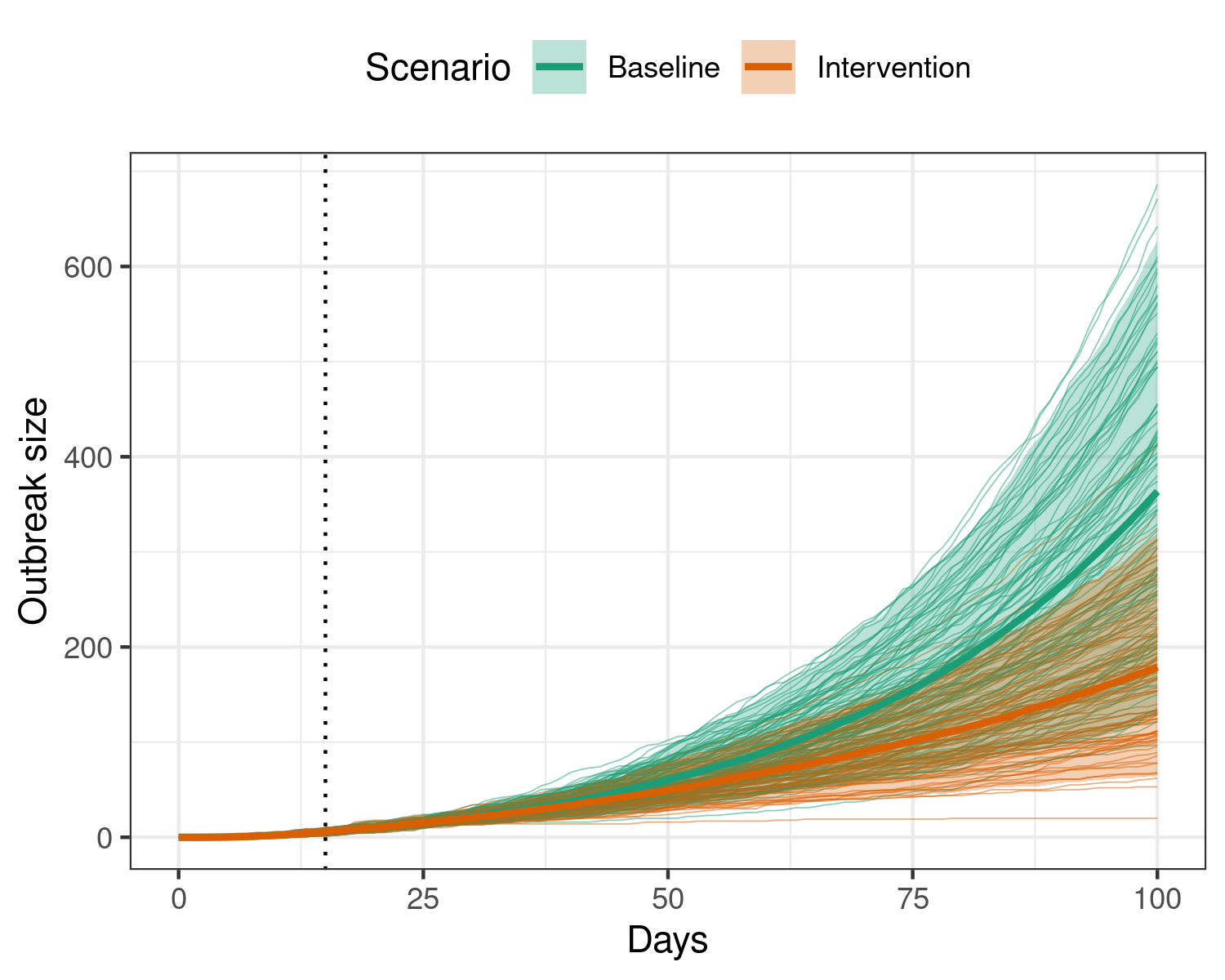
Figure 2: Effect of implementing an intervention that reduces transmission by 20% during an ebola outbreak. The intervention begins on the 15th day (dotted vertical line), and is active for the remainder of the model duration. Applying this intervention leads to many fewer individuals infectious with ebola over the outbreak.

We see that applying an intervention that reduces transmission may be effective in reducing outbreak sizes.

Modelling the roll-out of vaccination

We can also model the rollout of vaccination against EVD, but because this model is structured differently from other models in epidemics, vaccination must be modelled differently too.

model_ebola() does not accept a vaccination regime as a <vaccination> object, but we can still model the effect of vaccination as a gradual decrease in the transmission rate \(\beta\) over time.

This is done by using the time dependence functionality of epidemics.

New to implementing parameter time dependence in epidemics? It may help to read the vignette on time dependence functionality first!

Note that the time-dependence composable element cannot be passed as a set of scenarios.

We first define a function suitable for the time_dependence argument. This function assumes that the baseline transmission rate of ebola decreases over time, with a 0.5% reduction each day due to vaccination.

Code

# we assume a 0.5% daily reduction
# we assume that this vaccination begins on the 15th day
time_dep_vax <- function(
    time, x, time_start = 15, reduction = 0.005) {
  if (time < time_start) {
    x
  } else {
    x * (1.0 - reduction)^time
  }
}

Code

data_baseline <- with_seed(
  1,
  model_ebola(
    population = guinea_population
  )
)
data_vax_scenario <- with_seed(
  1,
  model_ebola(
    population = guinea_population,
    time_dependence = list(
      transmission_rate = time_dep_vax
    )
  )
)

data_baseline$scenario <- "baseline"
data_vax_scenario$scenario <- "scenario"

# bind the data together
data_scenarios <- bind_rows(data_baseline, data_vax_scenario)

Code

filter(data_scenarios, compartment == "removed") %>%
  ggplot(aes(time, value, colour = scenario)) +
  geom_vline(
    xintercept = 15,
    linetype = "dotted"
  ) +
  geom_line(
    aes(group = interaction(scenario, replicate)),
    linewidth = 0.2, alpha = 0.5
  ) +
  stat_summary(
    geom = "ribbon",
    fun.min = function(x) quantile(x, 0.025),
    fun.max = function(x) quantile(x, 0.975),
    alpha = 0.3, colour = NA,
    aes(fill = scenario)
  ) +
  stat_summary(
    geom = "line", linewidth = 1
  ) +
  scale_colour_brewer(
    palette = "Dark2",
    name = "Scenario",
    labels = c("Baseline", "Vaccination campaign")
  ) +
  scale_fill_brewer(
    palette = "Dark2",
    name = "Scenario",
    labels = c("Baseline", "Vaccination campaign")
  ) +
  theme_bw() +
  theme(
    legend.position = "top"
  ) +
  labs(
    x = "Days",
    y = "Outbreak size"
  )

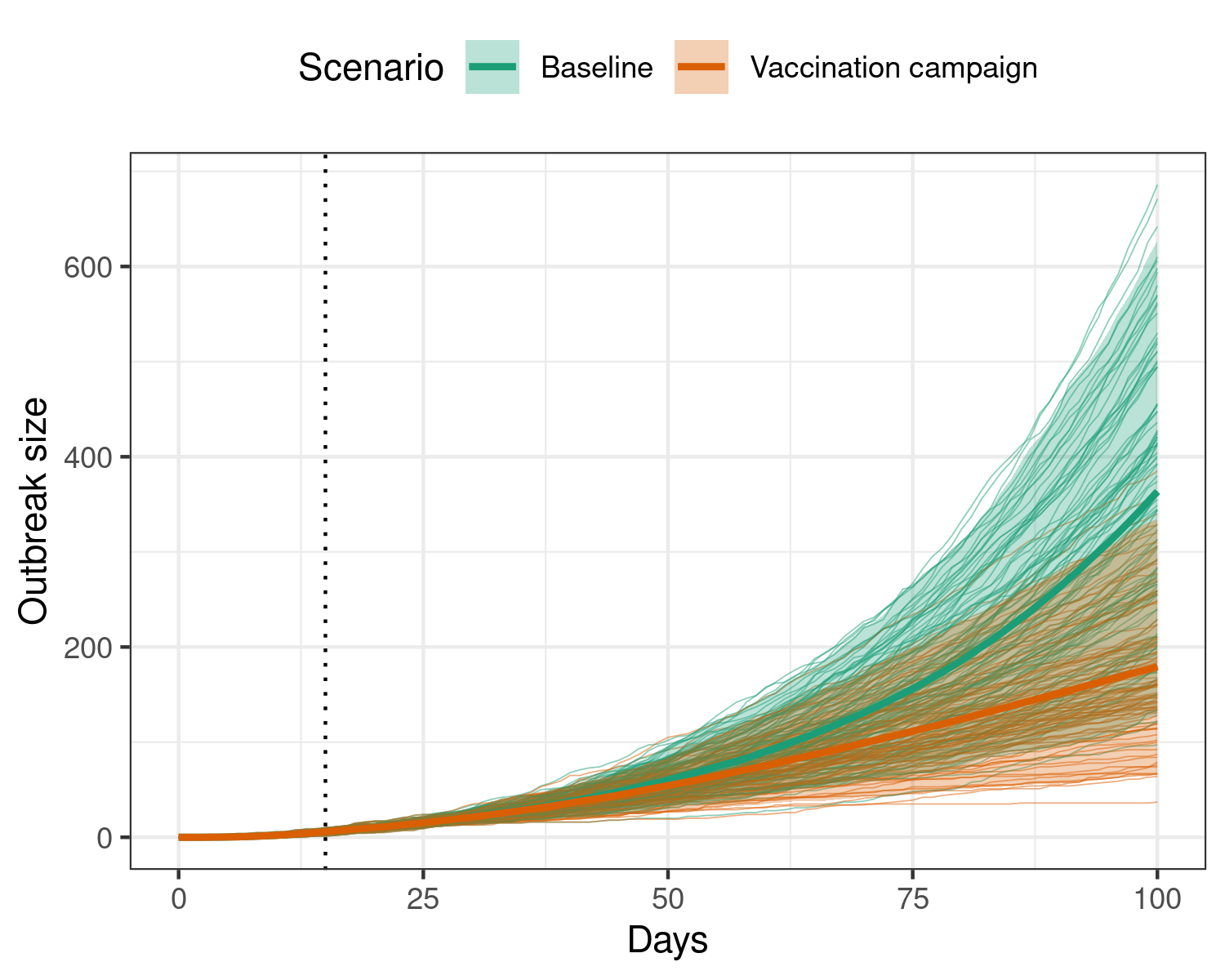
Figure 3: Effect of implementing a vaccination regime that gradually reduces ebola transmission over time, using the time dependence functionality.

Similar functionality can be used to model other parameters more flexibly than allowed by the <rate_intervention> class.

Modelling a multi-pronged ebola response

Since EVD is a severe disease with a high case fatality risk, responses to an outbreak may require the simultaneous implementation of a number of measures to reduce transmission to end the outbreak quickly.

We can use the EVD model and existing functionality in epidemics to model the implementation of a multi-pronged response to ebola that aims to improve:

• detection and treatment of cases,

• safety of hospitals and the risk of community transmission, and

• safety of funeral practices to reduce the risk of transmission from dead bodies.

Here, we show the combined effects of these interventions separately. We can pass the interventions to the model function’s intervention argument as a named list, with the names indicating the model parameters to target.

Code

# create an intervention on the transmission rate
improve_hospitalisation <- intervention(
  type = "rate",
  time_begin = 15, time_end = 100, reduction = 0.3
)

# create an intervention on ETU risk
improve_etu_safety <- intervention(
  type = "rate",
  time_begin = 15, time_end = 100, reduction = 0.7
)

# create an intervention on the transmission rate
reduce_funeral_risk <- intervention(
  type = "rate",
  time_begin = 15, time_end = 100, reduction = 0.5
)

Code

# create a list of single and combined interventions
intervention_scenarios <- list(
  baseline = NULL,
  combined = list(
    transmission_rate = reduce_transmission,
    prop_community = improve_hospitalisation,
    etu_risk = improve_etu_safety,
    funeral_risk = reduce_funeral_risk
  )
)

Code

# run the epidemic model and save data as the baseline, using a fixed seed
data_scenarios <- withr::with_seed(
  1,
  model_ebola(
    population = guinea_population,
    intervention = intervention_scenarios
  )
)

Code

# name the scenarios and unnest the data
data_scenarios <- mutate(
  data_scenarios,
  scenario = names(intervention_scenarios)
)

data_scenarios <- select(data_scenarios, scenario, data) %>%
  unnest(data)

Code

filter(data_scenarios, compartment == "removed") %>%
  ggplot(aes(time, value, colour = scenario)) +
  geom_vline(
    xintercept = 15,
    linetype = "dotted"
  ) +
  geom_line(
    aes(group = interaction(scenario, replicate)),
    linewidth = 0.2, alpha = 0.5
  ) +
  stat_summary(
    geom = "ribbon",
    fun.min = function(x) quantile(x, 0.025),
    fun.max = function(x) quantile(x, 0.975),
    alpha = 0.3, colour = NA,
    aes(fill = scenario)
  ) +
  stat_summary(
    geom = "line", linewidth = 1
  ) +
  scale_colour_brewer(
    palette = "Dark2",
    name = "Scenario",
    labels = c("Baseline", "Combined interventions")
  ) +
  scale_fill_brewer(
    palette = "Dark2",
    name = "Scenario",
    labels = c("Baseline", "Combined interventions")
  ) +
  theme_bw() +
  theme(
    legend.position = "top"
  ) +
  labs(
    x = "Days",
    y = "Outbreak size"
  )

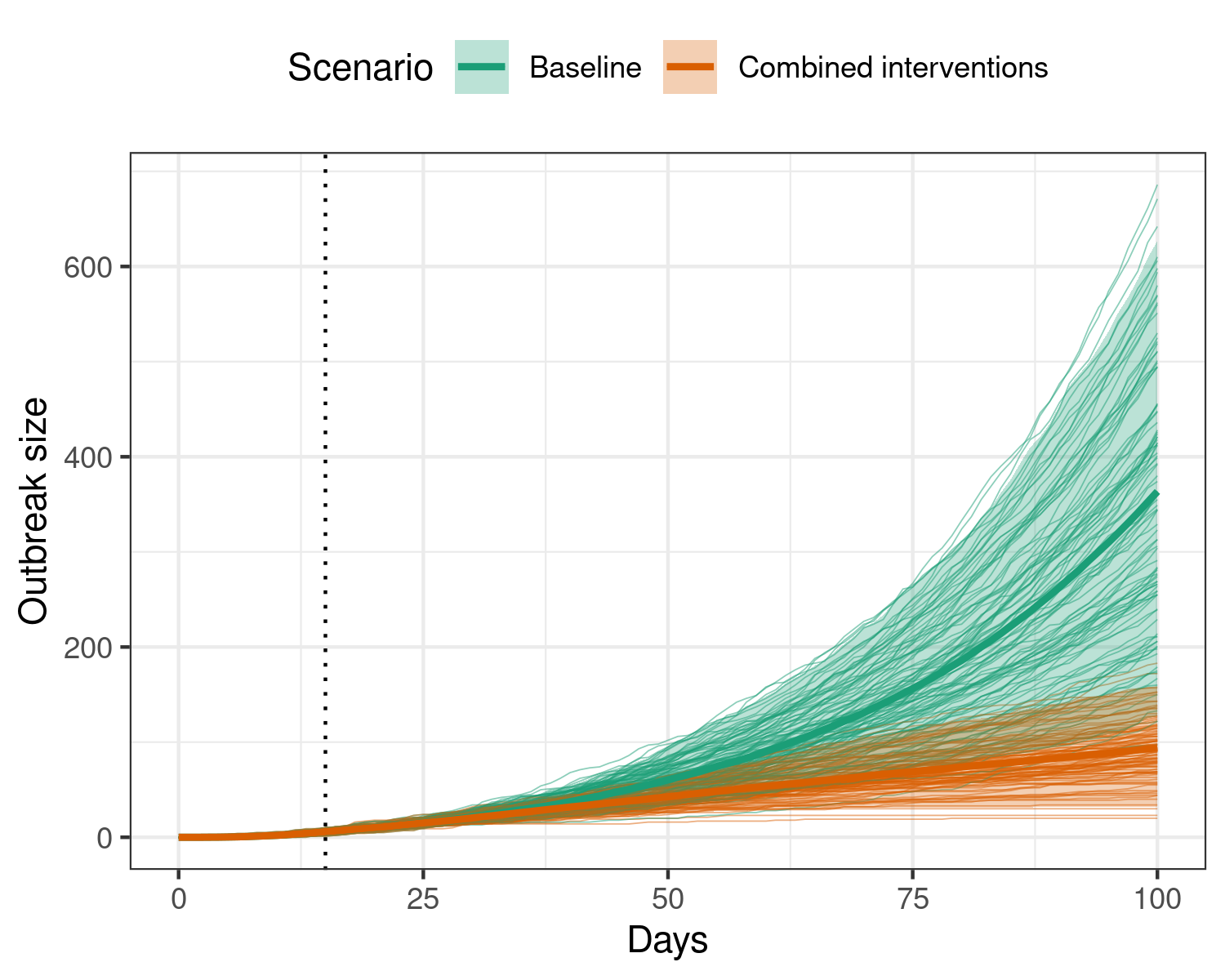
Figure 4: Effect of implementing multiple simultaneous interventions to reduce transmission during an ebola outbreak, all beginning on the 15th day (dotted vertical line), and remaining active for the remainder of the model duration. Applying these interventions substantially reduces the final size of the outbreak, with a potential plateau in the outbreak size reached at 100 days. Individual scenario replicates are shown in the background, while the shaded region shows the 95% interval, and the heavy central line shows the mean for each scenario.

Details: Discrete-time Ebola virus disease model

This model has compartments adopted from the consensus model for Ebola virus disease presented in Li et al. (2019), and with transitions between epidemiological compartments modelled using Erlang sub-compartments adapted from Getz and Dougherty (2018); see References.

The R code for this model is adapted from code by Ha Minh Lam and initially made available on Epirecipes under the MIT license.

The transition rates between the exposed and infectious, and infectious and funeral compartments (and also hospitalised to removed), \(\gamma^E\) and \(\gamma^I\) in Getz and Dougherty’s notation, are passed by the user as the infectiousness_rate and removal_rate respectively.

The shape of the Erlang distributions of passage times through the exposed and infectious compartments (\(k^E\) and \(k^I\)) are recommended to be set to 2 as a sensible choice, which is the default value for the erlang_sbubcompartments argument, but can be allowed to vary (but not independently).

Getz and Dougherty’s equation (6) gives the relationship between these parameters and the mean pre-infectious \(\rho^E\) and infectious \(\rho^I\) periods.

\[\gamma^E = \dfrac{k^E}{\rho^E} = \dfrac{2}{\rho^E} ~\text{and}~ \gamma^I = \dfrac{k^I}{\rho^I} = \dfrac{2}{\rho^I}\]

In this discrete time model, \(\gamma^E\) and \(\gamma^I\) are used to determine the passage times of newly exposed or infectious individuals through their respective compartments (thus allowing for variation in passage times).

Hospitalisation, funerals, and removal

Li et al. (2019) present a consensus model for EVD in which individuals can follow multiple pathways from the infectious compartment — to hospitalisation, funeral transmission, and safe burial or recovery (removed), with the possibility of skipping some compartments in this sequence (e.g. directly from infectious to removed, infectious to hospitalisation to removed etc.). This model simplifies these transitions to only two pathways:

1. Infectious → funeral → removed (safe burial)

2. Infectious → hospitalised → removed (recovery or safe burial)

A proportion, 1.0 - prop_community, of infectious individuals are transferred to the hospitalised compartment in each timestep, This compartment represents Ebola Treatment Units (ETUs), and individuals in the hospitalised compartment are considered to be infectious but no longer in the community.

The passage time of individuals in the hospitalised compartment is similar to that of individuals in the infectious compartment (i.e., infectious in the community), which means that an infectious individual with \(N\) timesteps before exiting the infectious compartment will exit the hospitalised compartment in the same time.

Hospitalised individuals can contribute to transmission of Ebola to susceptibles depending on the value of \(p_\text{ETU}\), which is the probability (or proportion) of hospitalised cases contributing to the infection of susceptibles. This is interpreted as the relative risk of Ebola virus treatment units (ETUs), with a range of 0.0 – 1.0, where 0.0 indicates that hospitalisation prevents onward transmission entirely, while 1.0 indicates that hospitalisation does not reduce transmission at all. This is passed as the argument etu_risk.

We assume that deaths in hospital lead to Ebola-safe funerals, and individuals exiting the hospitalised compartment move to the ‘removed’ compartment, which holds both recoveries and deaths.

We assume that infectious individuals who are not hospitalised die, and that deaths outside of hospital lead to funerals that are potentially not Ebola-safe, and the contribution of funerals to Ebola transmission is determined by \(p_\text{funeral}\), which can be interpreted as the relative risk of funerals, and is passed as the funeral_risk argument. Values closer to 0.0 indicate that there is low to no risk of Ebola transmission at funerals, while values closer to 1.0 indicate that the risk is similar to that of transmission in the community.

Individuals are assumed to spend only a single timestep in the funeral transmission compartment, before they move into the ‘removed’ compartment. Individuals in the ‘removed’ compartment do not affect model dynamics.

References

Althaus, Christian L. 2014. “Estimating the Reproduction Number of Ebola Virus (EBOV) During the 2014 Outbreak in West Africa.” PLoS Currents 6 (September): ecurrents.outbreaks.91afb5e0f279e7f29e7056095255b288. https://doi.org/10.1371/currents.outbreaks.91afb5e0f279e7f29e7056095255b288.

Getz, Wayne M., and Eric R. Dougherty. 2018. “Discrete Stochastic Analogs of Erlang Epidemic Models.” Journal of Biological Dynamics 12 (1): 16–38. https://doi.org/10.1080/17513758.2017.1401677.

Li, Shou-Li, Matthew J. Ferrari, Ottar N. Bjørnstad, Michael C. Runge, Christopher J. Fonnesbeck, Michael J. Tildesley, David Pannell, and Katriona Shea. 2019. “Concurrent Assessment of Epidemiological and Operational Uncertainties for Optimal Outbreak Control: Ebola as a Case Study.” Proceedings of the Royal Society B: Biological Sciences 286 (1905): 20190774. https://doi.org/10.1098/rspb.2019.0774.